Abstract: This project explores CLIP - Contrasive Language-Image Pre-training, a pre-training technique that jointly trains image and text encoders to map them into the same feature space. This project reproduces CLIP’s one shot ability and performance of a linear classifier using CLIP’s features. It also proposes a method to initialize the few-shot classifiers, solving the previously discovered problem that few-shot classifiers could underperform zero-shot classifier. It is found that there is a special type of overfitting in few-shot classification, which poses a significant challenge to the concept of few-shot classification. This project also trains a image generation model and a semantic segmentation model using CLIP’s features, which can provide us insight into the amount of information that CLIP’s features contain.

• Introduction
  • How CLIP Works
  • Technical Details
    • The Contrasive Loss Function
  • The Algorithm
• Our Experiments
  • Fine tuning CLIP with a Linear Classifier
    • Discussion
  • Zero-Shot Classification with CLIP
    • Discussion
  • Solving the problem of few shot Performance
    • Motivation
    • Method
    • Results
    • Discussion
  • Training a Decoder using CLIP’s Features
    • Motivation
    • Method
    • Results
    • Discussion
  • Training Segmentation from CLIP
    • Motivation
    • Method
    • Results
    • Discussion
• Conclusion
• Spotlight Presentation
  • Reference

Introduction

The goal of this project is to explore and understand CLIP - Contrasive Language-Image Pre-training.

Before CLIP, although there have been a lot of models in computer vision that achieve very good performances, they typically requires large amount of labeled data and are trained only to perform well in one specific task. For example, for image classification task, there needs to be someone who assign each image in the dataset a label in a predefined format. It would be great if one can utilize the vast amount of text-image pair on the internet, though they are not labeled in some strict format. In addition, after training a model on such dataset, the model would not work on another dataset labeled in a different way. It will also not recognize new types of objects, unless we train with a lot of additional data on that object.

CLIP is able to solve these problems by jointly training image encoder and text encoder. It is able to train a model that can move to a task that it has not seen before without large amount of extra data. It is worth noting that CLIP is a pre-training technique: it does not directly optimize towards specific task such as classfication or object detection. Rather, it contains a text encoder and an image encoder that maps texts and images to the same feature space. The text and features that are close in the feature space are considered to be representing similar concepts.

CLIP also has a number of limitations. According to “Learning Transferable Visual Models From Natural Language Supervision” ¹, CLIP struggles in performing more abstract tasks, such as counting the number of objects. Also, when fine-tuning CLIP on a dataset using only a few images per class, the performance actually get worse.

For our project, we want to run the code for CLIP on our own and explore its properties. We will also explore the limitations mentioned above: why they are happening and whether we can solve them.

How CLIP Works

CLIP is a method to pretrain a model. CLIP trains a network that extracts features from an image, whose results can be used for later layers to do image classification.

CLIP trains an image encoder and a text encoder. “Encoders” mean networks that map the input image to a vector. The goal is to use the image encoder and the text encoder to map the images and texts to the same space – so that the same vector can represent key features from both images and texts.

CLIP is particularly good for “zero-shot” training. “Zero-shot” refers to the ability of a model to generalize to a different context without any additional training data.

Technical Details

The Contrasive Loss Function

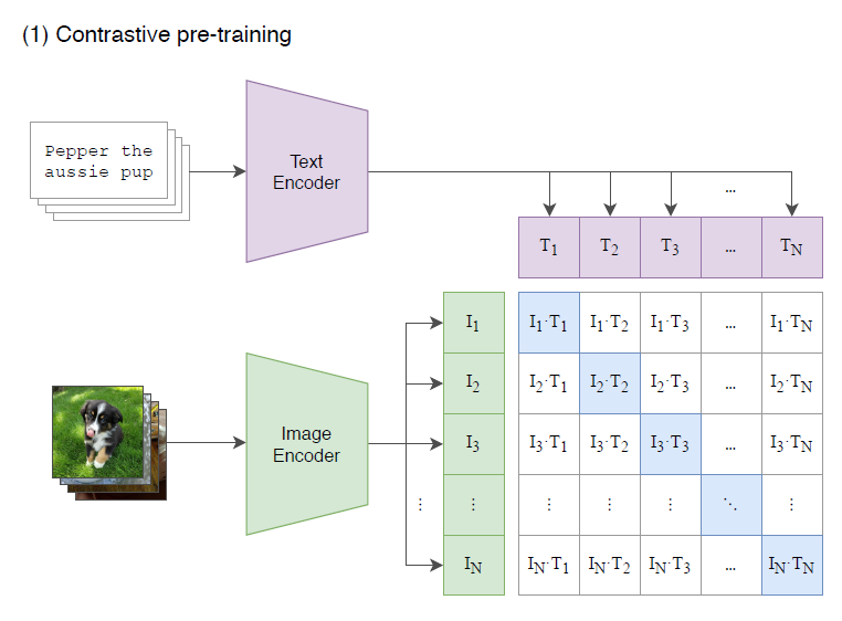
Fig 1. CLIP’s pretraining process ¹

The training process is contrasive. As shown in the above figure from “Learning Transferable Visual Models From Natural Language Supervision” ¹, the image encoder and the text encoder are trained together to maximize the cosine similarity between image_encoder(image) and text_encoder(text) of a correct (image, text) pair in the dataset. The actual loss function captures this metric. The loss function has two parts, calculating cross entropy loss from two directions. The first part calculates distances from each encoded image to all the encoded texts, and calculate the cross entropy loss between such distances and the correct text associated with this image. The second part calculates distances from each encoded text to all the encoded images, and calculate the cross entropy loss between such distances and the correct image associated with this text. The actual loss is the average of the two.

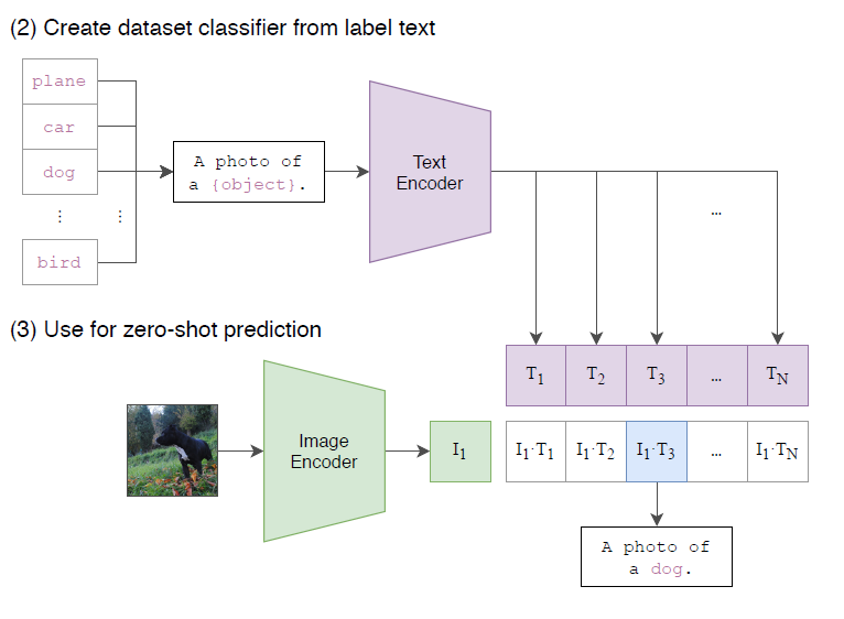
Fig 2. Zero-shot classification with CLIP ¹

As can be seen from the description about, the cosine similarity between the text feature and the image feature will then represent how close they are in the feature space. Then this will provide an obvious method for “zero-shot” classfication. As shown in the figure above, from “Learning Transferable Visual Models From Natural Language Supervision”¹, we can first map all the labels to there feature space using the text encoder. Then, for any input image, we may encode it, and compute its cosine similarity with all the labels, and pick the one with the highest similarity as the prediction.

The Algorithm

The algorithm for training loss is as follows: ¹

# image_encoder - ResNet or Vision Transformer
# text_encoder - CBOW or Text Transformer
# I[n, h, w, c] - minibatch of aligned images
# T[n, l] - minibatch of aligned texts
# W_i[d_i, d_e] - learned proj of image to embed
# W_t[d_t, d_e] - learned proj of text to embed
# t - learned temperature parameter
# extract feature representations of each modality
I_f = image_encoder(I) #[n, d_i]
T_f = text_encoder(T) #[n, d_t]
# joint multimodal embedding [n, d_e]
I_e = l2_normalize(np.dot(I_f, W_i), axis=1)
T_e = l2_normalize(np.dot(T_f, W_t), axis=1)
# scaled pairwise cosine similarities [n, n]
logits = np.dot(I_e, T_e.T) * np.exp(t)
# symmetric loss function
labels = np.arange(n)
loss_i = cross_entropy_loss(logits, labels, axis=0)
loss_t = cross_entropy_loss(logits, labels, axis=1)
loss = (loss_i + loss_t)/2

There are models in computer vision and natural language processing that can be used as encoders. The image encoder is based on either ResNet or Transformer and the text encoder is based on Transformer.

Our Experiments

We did several experiments with CLIP to explore its properties. This section also includes our innovations.

Fine tuning CLIP with a Linear Classifier

To begin, we run the example code at https://github.com/openai/CLIP. We first configure the environment by running

$ conda install --yes -c pytorch pytorch=1.7.1 torchvision cudatoolkit=11.0
$ pip install ftfy regex tqdm
$ pip install git+https://github.com/openai/CLIP.git

Then, using the example code we train a logistic regression model above the pretrained CLIP model to do image classification. We only update the parameters of the logistic model, without fine tuning the parameters of the encoders. The code is as follows:

import os
import clip
import torch

import numpy as np
from sklearn.linear_model import LogisticRegression
from torch.utils.data import DataLoader
from torchvision.datasets import CIFAR100
from tqdm import tqdm

# Load the model
device = "cuda" if torch.cuda.is_available() else "cpu"
model, preprocess = clip.load('ViT-B/32', device)

# Load the dataset
root = os.path.expanduser("~/.cache")
train = CIFAR100(root, download=True, train=True, transform=preprocess)
test = CIFAR100(root, download=True, train=False, transform=preprocess)


def get_features(dataset):
    all_features = []
    all_labels = []
    
    with torch.no_grad():
        for images, labels in tqdm(DataLoader(dataset, batch_size=100)):
            features = model.encode_image(images.to(device))

            all_features.append(features)
            all_labels.append(labels)

    return torch.cat(all_features).cpu().numpy(), torch.cat(all_labels).cpu().numpy()

# Calculate the image features
train_features, train_labels = get_features(train)
test_features, test_labels = get_features(test)

# Perform logistic regression
classifier = LogisticRegression(random_state=0, C=0.316, max_iter=1000, verbose=1)
classifier.fit(train_features, train_labels)

# Evaluate using the logistic regression classifier
predictions = classifier.predict(test_features)
accuracy = np.mean((test_labels == predictions).astype(float)) * 100.
print(f"Accuracy = {accuracy:.3f}")

We are able to get the following result:

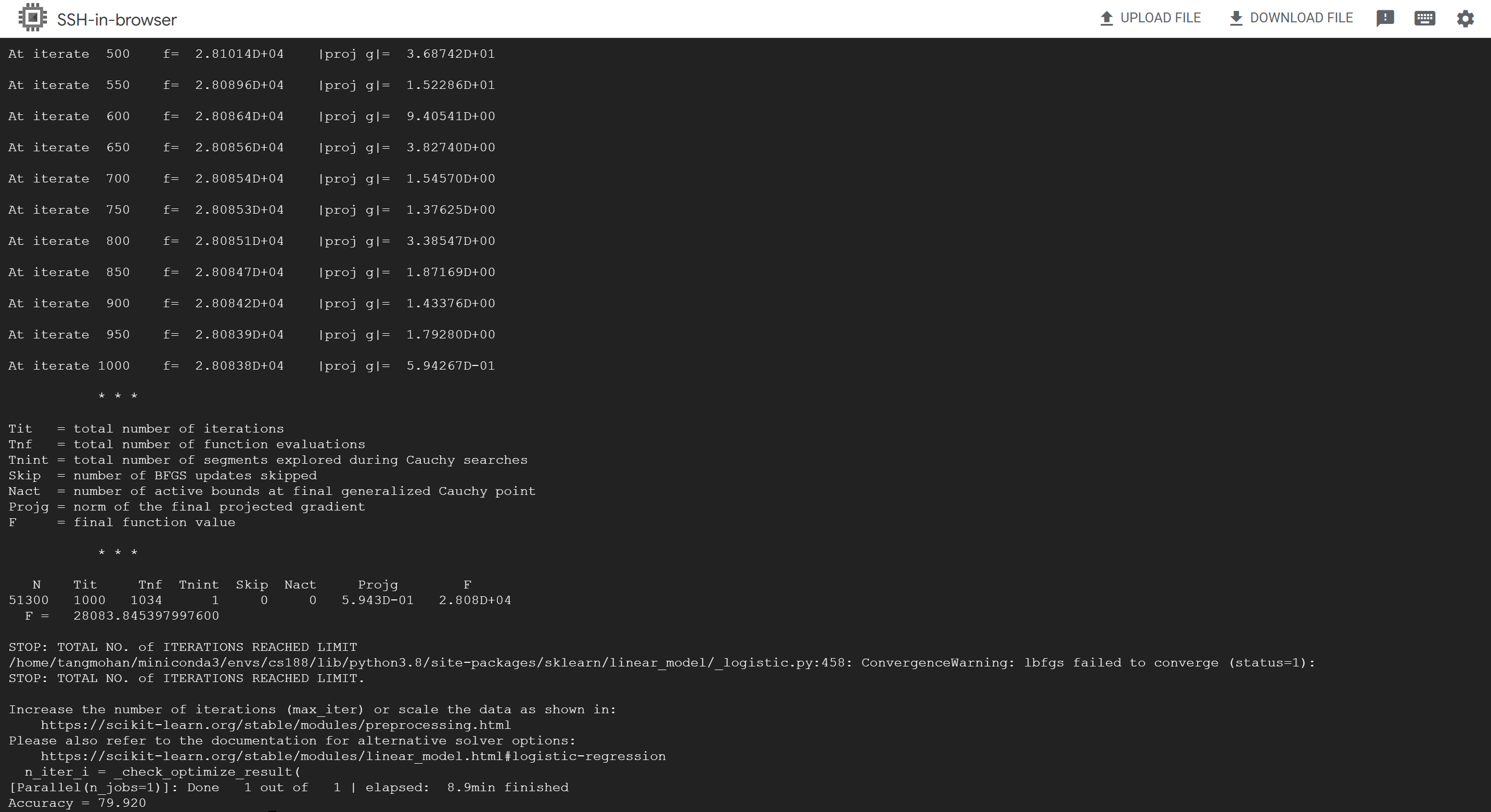
Fig 3. Training a linear classifier with CLIP’s features

Discussion

The accuracy is 79.920. This is better than ResNet-1001 on CIFAR 100, which is the dataset used. As we know, the linear regression model is a very simple model, so this is showing the generalizability of CLIP – trained on one dataset, it is able to generalize to a different context with small amount of additional training.

Zero-Shot Classification with CLIP

We also test CLIP’s zero-shot ability on the testing set of CIFAR100. This is the code that we use:

model, preprocess = clip.load('ViT-B/32', device)
cifar100 = CIFAR100(root=os.path.expanduser("~/.cache"), download=True, train=False)
text_inputs = torch.cat([clip.tokenize(f"a photo of a {c}") for c in cifar100.classes]).to(device)
with torch.no_grad():
    text_features = model.encode_text(text_inputs)
text_features /= text_features.norm(dim=-1, keepdim=True)

import torch.nn as nn
class ZeroShot(nn.Module):
    def __init__(self):
        super().__init__()

    def forward(self, x):
        x = model.encode_image(x)
        x = x / x.norm(dim=-1, keepdim=True)
        #return self.fc2(self.relu(self.fc1(x)))
        return x@text_features.T

Discussion

Evaluating this model, we obtain an accuracy of 0.6168. This is a pretty high number, showing the zero-shot ability of CLIP.

Solving the problem of few shot Performance

Motivation

In the paper that introduces CLIP, “Learning Transferable Visual Models From Natural Language Supervision”, the authors notes that, counter to there expectation, few-shot CLIP – linear classifier using CLIP’s features trained with only a few samples from each class – significantly underperforms zero-shot CLIP when the number of samples for each class is less than 4. With more examples to train with, why does few shot classifiers get worse than zero-shot classfier? The authors proposed that the when training few-shot CLIPs, we are using treating each label just as a separate dimension to be used in a logistic model, thereby discarding the information about the label’s texts that the zero-shot CLIP contains. The authors couldn’t find a way to solve this problem, and considered it a promising direction for future work. This is the plot illustrating their finding, obtained from CLIP’s original paper. ¹

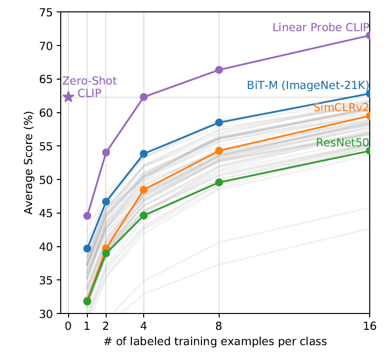
Fig 4. Few-shot underperform zero-shot ¹

Method

Our method comes from the idea that the zero-shot classifier itself is just a linear classifier on the features of CLIP, so we may initialize our linear classifier to match the zero-shot classifier.

The zero-shot classifier is given by the following formula. For an image \(x\) if we use \(P\) to represent the probability for different classes, then

where @ represents matrix multiplication.

The formula for linear classifiers is as follows:

where \(L\) is a linear transformation.

Therefore, in order to initialize the linear classifier to the zero-shot classifier, for the linear classifier \(L(v) = v @ W^T + b\), we just need to let \(W = encodetext(ClassLabels)\) and \(b = 0\).

This is our code:

model, preprocess = clip.load('ViT-B/32', device)
class Clip_Plus_MLP(nn.Module):
    def __init__(self, weights, zero_shot_initialization = True):
        super().__init__()
        self.clip = model.visual
        for param in self.clip.parameters():
            param.requires_grad = False
        self.fc1 = torch.nn.Linear(512, 100)           
        if(zero_shot_initialization):        
          self.fc1.weight.data = weights.clone()
          nn.init.constant_(self.fc1.bias, 0)
        self.fc1 = self.fc1.half()

    def forward(self, x):
        x = self.clip(x.type(model.dtype))
        x = x / x.norm(dim=-1, keepdim=True)
        return self.fc1(x)

Results

Testing our method on CIFAR100’s testing dataset, using this initialization without further training, we get an accuracy of 0.6168, which match the accuracy of zero-shot CLIP (as expected).

Now what happens when we use this initialization on few-shot classification? We obtain the following plot.

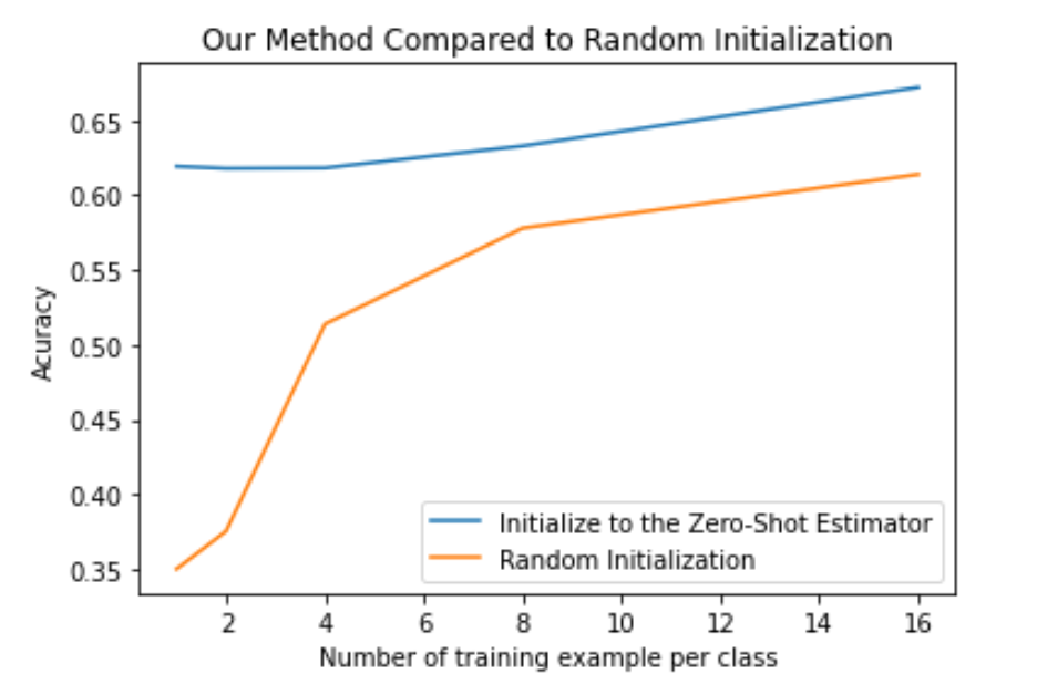
Fig 5. Improvement on Few Shot Performance

Discussion

We can see that for random initialization, 1 shot prediction underperforms zero-shot prediction by a lot, and the accuracy increases only after the number of training examples increases, just as what is shown in “Learning Transferable Visual Models From Natural Language Supervision” ¹. We see that with our initialization, the problem previously mentioned is gone. One-shot accuracy is no longer below zero-shot accuracy.

However, it isn’t performing too much better than the zero-shot classifier either. To understand the reason why this happens, we examines how validation accuracy changes with time when we train the one-shot classifier. We obtain the following plot:

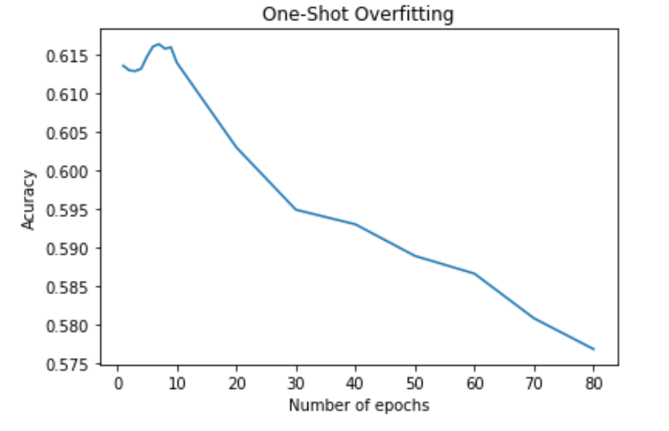
Fig 6. One shot validation accuracy vs number of epochs

It can be seen that validation accuracy starts dropping almost immediately after we start training. This is strongly suggesting that we are actually overfitting. On a second thought, this seems to be the reasonable outcome. As an example, an image of a dog may be best matched to the text “a sleeping dog” using CLIP, whereas another image may be best matched to the text “a running dog”. However, when doing classification, both images may be labeled as just “dog” in the training set. Therefore, each class in the training dataset may have different modes. However, doing few-shot training, the examples only provide us with information about limited number of modes for each class. For example, if we are doing one-shot training, we may get an image of a sleeping dog for the class “dog”, and we may learn a template for the sleeping dogs instead of the whole class “dog”. If this is the case, then the more we train, the more we are learning a template that suits just the training examples provided intead of the whole class. The accuracy inceases as the number of examples increases, possibly because now the examples can provide information about more modes for each class. This may be a fundamental challenge for few-shot training. Nevertheless, our initialization method makes sure that few-shot classification is a least as good as zero-shot classification.

Training a Decoder using CLIP’s Features

Motivation

In “Learning Transferable Visual Models From Natural Language Supervision”, the authors notes that zero-shot CLIP struggles at complex tasks such as perdicting the number of objects or distance between objects. ¹

In this section, we are going to explore this problem indirectly. One possible cause for the problem is that the CLIP’s encoder lose the information about number of objects and distance when encoding. Therefore, we want to have a look at how much information CLIP’s encoder actually contain.

We are going to train a generative model based on CLIP. We use the generative model VQ-VAE, but replace the encoder by CLIP’s image encoder. Freezing the encoder, we train the decoder to recover the original image.

By looking at the performance of such generator, we may see how much information CLIP’s feature contain, in comparison to the amount of information contained by VQVAE’s feature. Will we be able to recover the original image from CLIP’s fe-ature?

Method

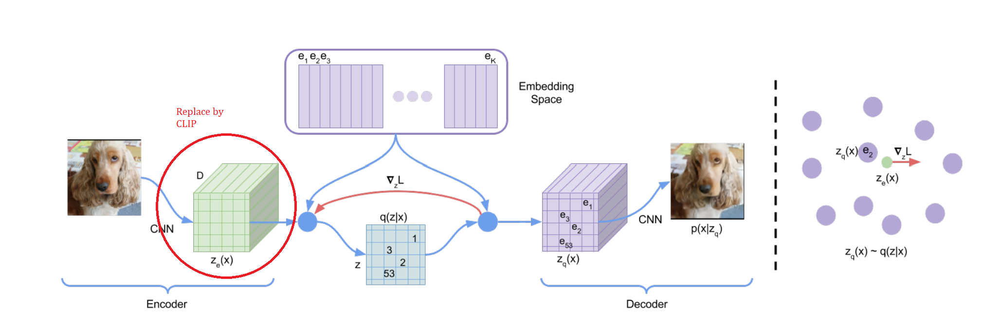
Fig 7. Graph illustration of VQ-VAE ²

VQ-VAE is a modified version of the VAE model that we covered in class. As shown in the above figure, from “Neural Discrete Representation Learning “ ², in comparison to VAE, there is an additional discretization step between the encoder and decoder, making the distribution of feature \(z\) discret.

In our experiment, we are replacing the encoder part with CLIP’s image encoder. However, we need to make a modification to CLIP’s encoder as well.

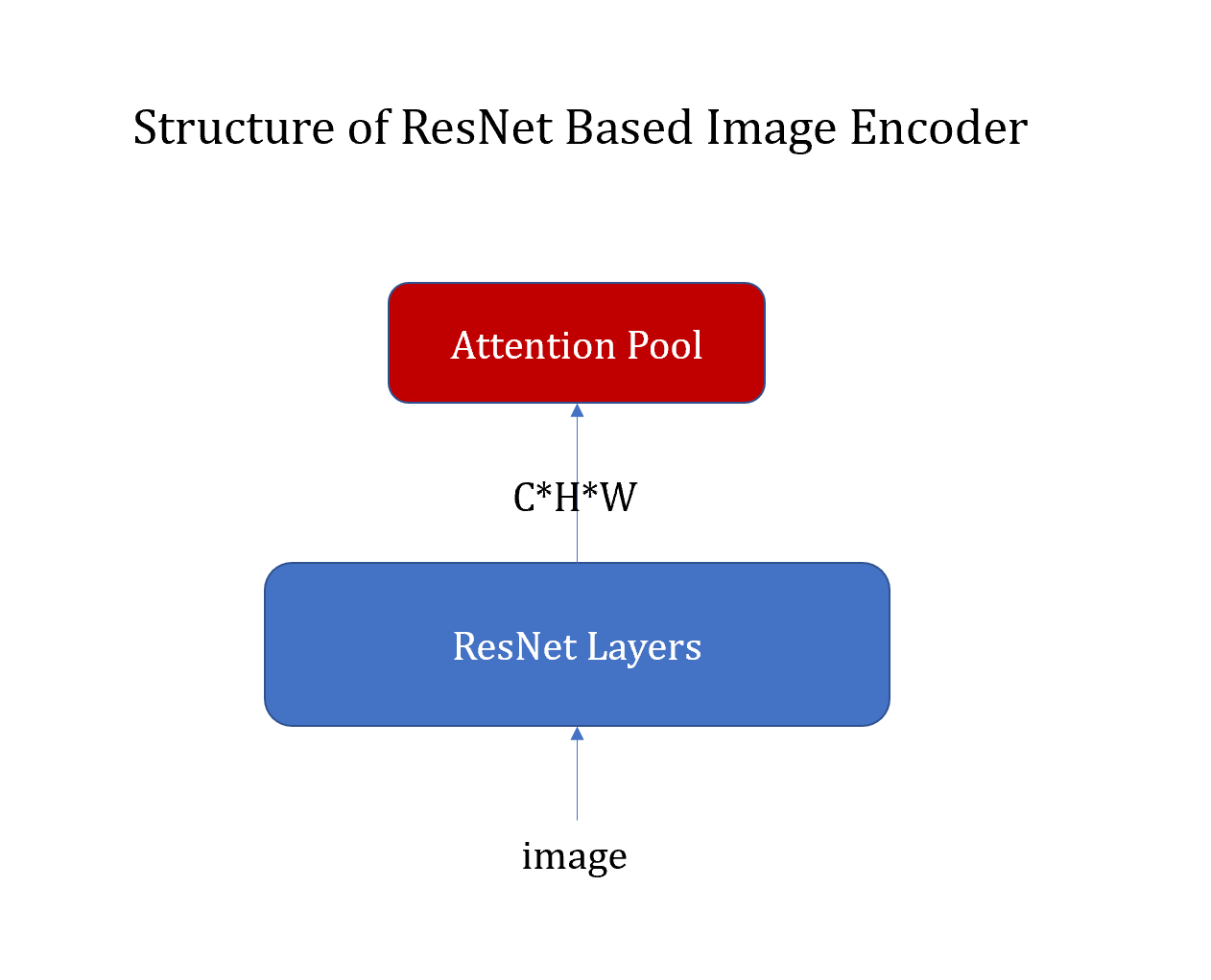
Fig 8. Structure of ResNet based CLIP

ResNet based CLIP has a structure shown in the image above. The output of ResNet Layers has the dimension \(C \times H \times W\). There is a final attention pool layer that takes each pixel as a token and output a 1-d vector of width \(C\).

The final output is a flattened vector, so it would be hard to extract spacial information from it. Therefore, we remove the attention layer, and feed the feature of size \(C \times H \times W\) to the later parts of the VQ-VAE network.

This is our code:

class CLIP_Encoder(nn.Module):
    def __init__(self):
        super().__init__()
        self.clip = cl_model.visual
        for param in self.clip.parameters():
            param.requires_grad = False 
        self.clip.attnpool = torch.nn.Identity() 
        self.pool =  nn.Conv2d(CLIP_dim, hidden_dim,1)

    def forward(self, x):                
        return self.pool(self.clip(x.type(cl_model.dtype)).float())

encoder = CLIP_Encoder()
codebook = VQEmbeddingEMA(n_embeddings=n_embeddings, embedding_dim=hidden_dim)
decoder = Decoder(input_dim=hidden_dim, hidden_dim=hidden_dim, output_dim=output_dim)

model = Model(Encoder=encoder, Codebook=codebook, Decoder=decoder).to(DEVICE)

Here the ‘VQEmbeddingEMA’ and ‘Decoder’ modules are the modules from VQ-VAE network, obtained from example pytorch implementation of VQ-VAE by Minsu Kang ³.

Note that with our modification the size of outputs will be changed as well. Therefore we need to resize the labels (the images themselves) during the training process.

Results

We use ResNet-50 based CLIP. In this case, the output of CLIP’s image encoder has input dimension \(3\times 224 \times 224\), and output dimension \(2048\times 7\times 7\). The output of the decoder has dimension \(3\times 28\times 28\).

Training our model, we can generate the following images from CLIP’s feature (using encoding of actual images). We can compare them to the ground truth images used. Note that those examples are from the testing set.

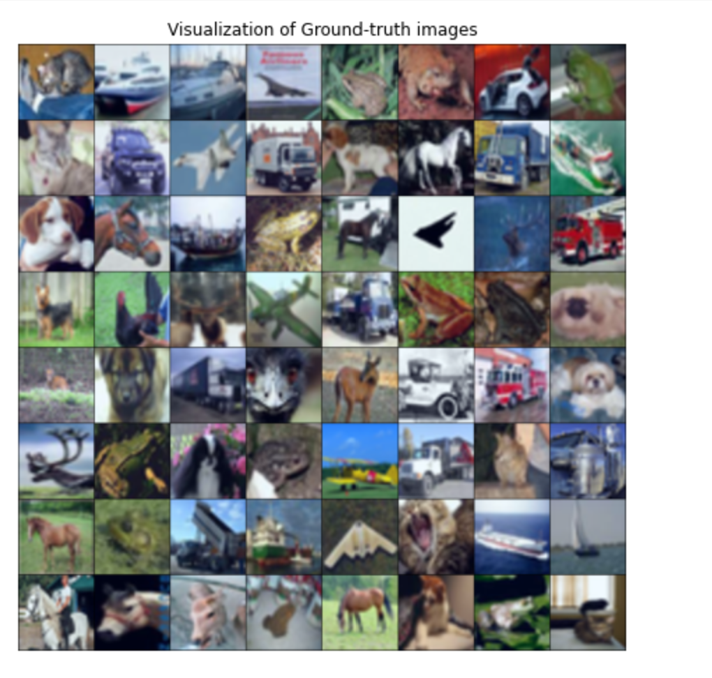
Fig 9. Ground Truth Images

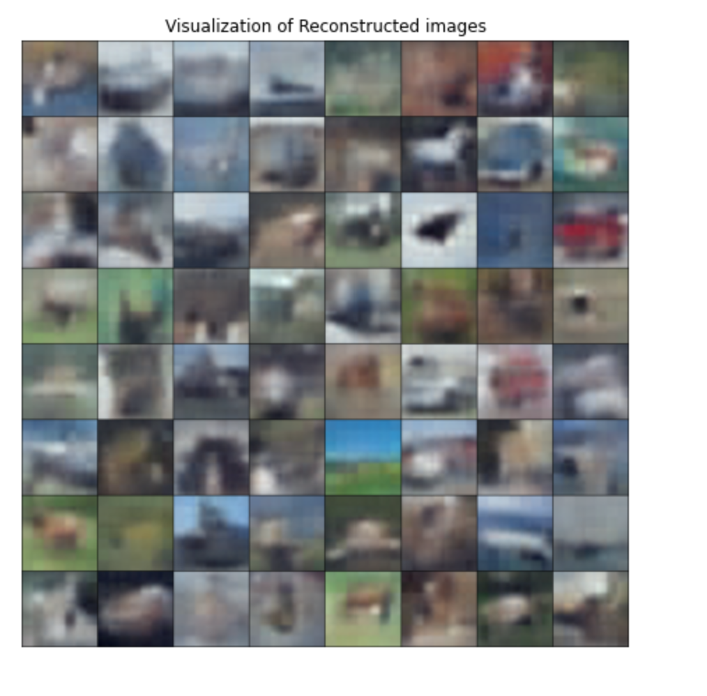
Fig 10. Reconstruction from CLIP’s Based Generator

We may also compare this with the result of the sample VQ-VAE model³.

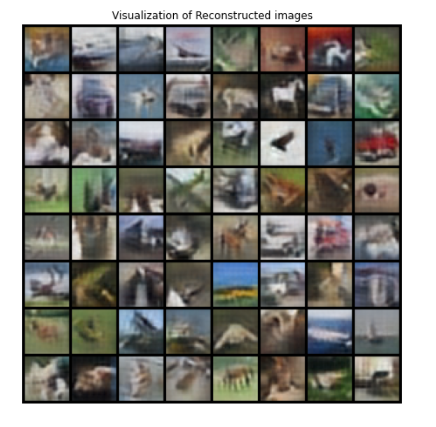
Fig 11. Reconstruction from VQ-VAE Example

Discussion

For both models, the performance of the decoder using random latent code is pretty bad. Here is an example:

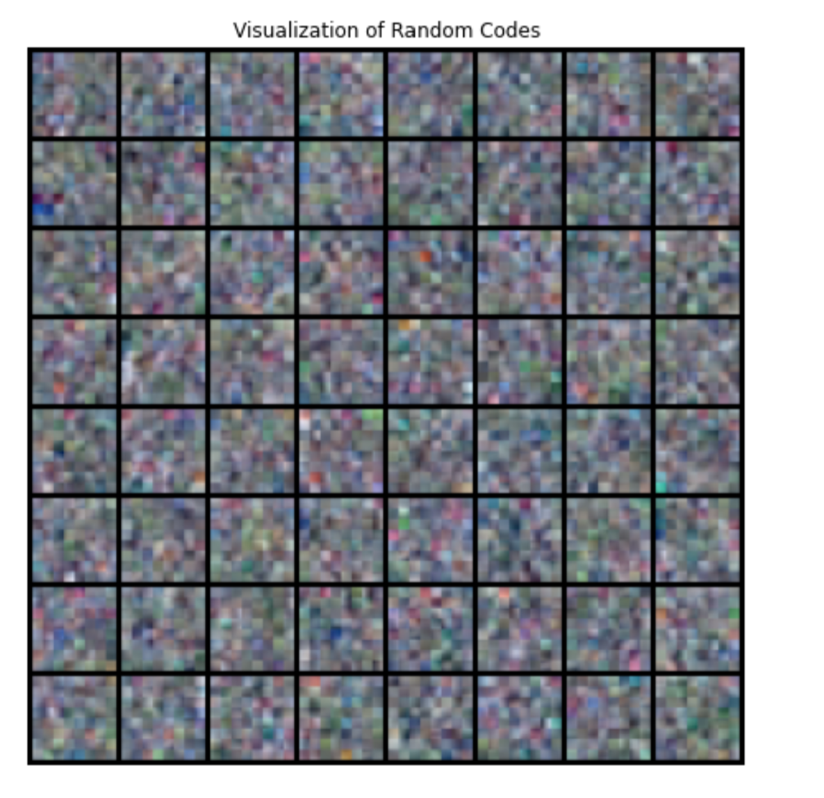
Fig 12. Generation from Random Code

This is probably because the models are too simple to generate completely new images. Nevertheless, the purpose of this experiment is to compare the information loss of the encoder of CLIP and that of the encoder of VQ-VAE.

We can see that the result using CLIP’s encoder is quite blur in comparison to the result from VQ-VAE’s original encoder as well as the ground truth. Therefore, it seems that feature from CLIP’s image encoder does not have as much information as feature from trained encoder of VQ-VAE.

We can also infer this from the training loss. Using our model, the training loss at the last epoch is 1.7655, whereas the training loss for the original model at the last epoch is 0.1265.

However, it is worth noting that the genenerator trained on CLIP still captures the rough shapes and colors of objects. This tell us the CLIP’s image encoder does preserve information about colors as well as positions (before the attention pool), as CLIP’s output is the only source fed to later parts of the generator.

Can we conclude from here that feature from CLIP’s image encoder does not have enough information to perform well on abstract tasks? We might need to look closer. Generators need information to help them predict the visual details of a image, which might not be neccessary for language related tasks. This motivates the following experiment.

Training Segmentation from CLIP

Motivation

This is another way that we are trying to see the information contained by CLIP’s features. We will train a decoder which take input from CLIP’s encoder, which will predict masks of objects. Intuitively, abstract tasks such as predicting the number of objects and predicting the distance between objects involve information about what the objects are and where they are. Therefore, the performance of CLIP’s encoder in a downstream task of segmentation should better represent whether it preserves enough information for those abstract tasks.

Using CLIP’s feature, we will train a decoder that do sementic segmentation, without modifying the parameters of CLIP.

Method

Same as before, we remove the last attention pool layer from CLIP’s image encoder. We want to freeze the encoder when training.

For the decoder, our code is based on semantic segmentation example provided by Tramac⁴, which is based on UNet11 model by Vladimir Iglovikov ⁵.

This is our modification:

class CLIP_seg(nn.Module):
    def __init__(self) -> None:
        super().__init__()
        self.clip = cl_model.visual
        cl_model.visual.attnpool = torch.nn.Identity()
        self.seg_model = create_model(params)
        for param in self.clip.parameters():
            param.requires_grad = False 
        for param in self.seg_model.parameters():
            param.requires_grad = False 
        self.center = self.seg_model.center
        self.dec5 = self.seg_model.dec5
        self.dec4 = self.seg_model.dec4
        self.dec3 = self.seg_model.dec3
        self.dec2 = self.seg_model.dec2
        self.dec1 = self.seg_model.dec1

        self.final = self.seg_model.final

        self.dec5.requires_grad = True
        self.dec4.requires_grad = True
        self.dec3.requires_grad = True
        self.dec2.requires_grad = True
        self.dec1.requires_grad = True
        self.center.requires_grad = True
        self.pool = nn.MaxPool2d(2, 2)

        self.final.requires_grad = True
        self.unpool5 = DecoderBlock(
            2048, 1280, 512
        )
        self.unpool4 = DecoderBlock(
            512, 512, 512
        )
        self.unpool3 = DecoderBlock(
            512, 512, 256
        )
        self.unpool2 = DecoderBlock(
            256, 256, 128
        )
        self.unpool1 = DecoderBlock(
            128, 128, 64
        )
        

    def forward(self, x: torch.Tensor) -> torch.Tensor:
        conv5 = self.clip(x.type(cl_model.dtype))
        conv5 = self.unpool5(conv5.float())
        conv4 = self.unpool4(conv5)
        conv3 = self.unpool3(conv4)
        conv2 = self.unpool2(conv3)
        conv1 = self.unpool1(conv2)

        center = self.center(self.pool(conv5.float()))

        dec5 = self.dec5(torch.cat([center, conv5], 1))
        dec4 = self.dec4(torch.cat([dec5, conv4], 1))
        dec3 = self.dec3(torch.cat([dec4, conv3], 1))
        dec2 = self.dec2(torch.cat([dec3, conv2], 1))
        dec1 = self.dec1(torch.cat([dec2, conv1], 1))
        return self.final(dec1) 

where ‘create_model’ creates a UNet11 segmentation model including the encoder and the decoder. We extract the decoder part of it. However, the decoder also uses residual blocks, taking inputs from different convolutional layers before. Here we just replace all of them with tensors obtained by upsampling CLIP’s feature.

In addition, we change resize the images to \(224\times 224\), fitting the size of input of CLIP. The output happens to have size \(224\times 224\) as well.

Results

After training (10 epochs), below are the masks that the model generates on the testing set. We can compare them with the ground truth.

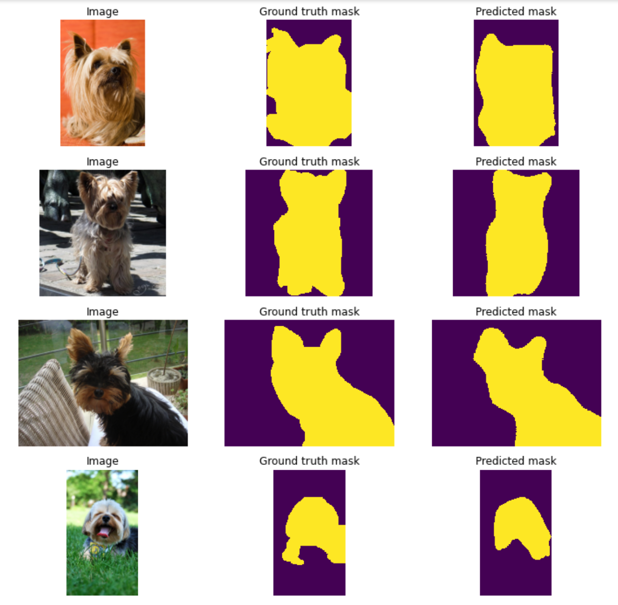
Fig 13. Clip-based segmentation result

We can also compare the validation loss of CLIP based segmentation and the validation loss of the original model.

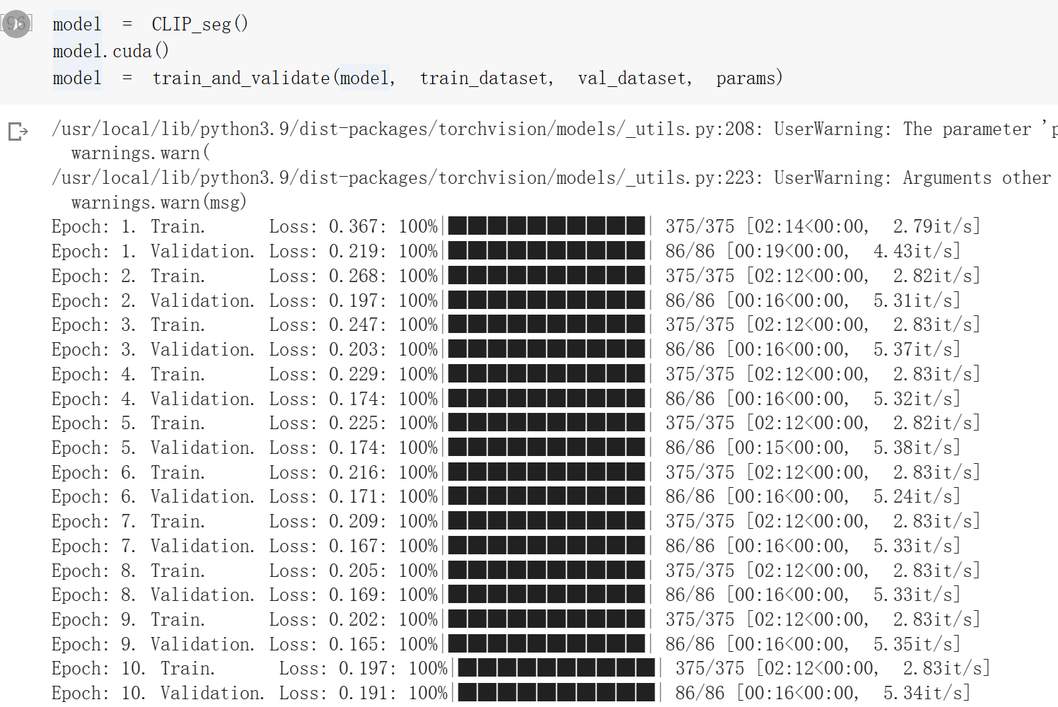
Fig 14. Validation loss of CLIP-based segmentation

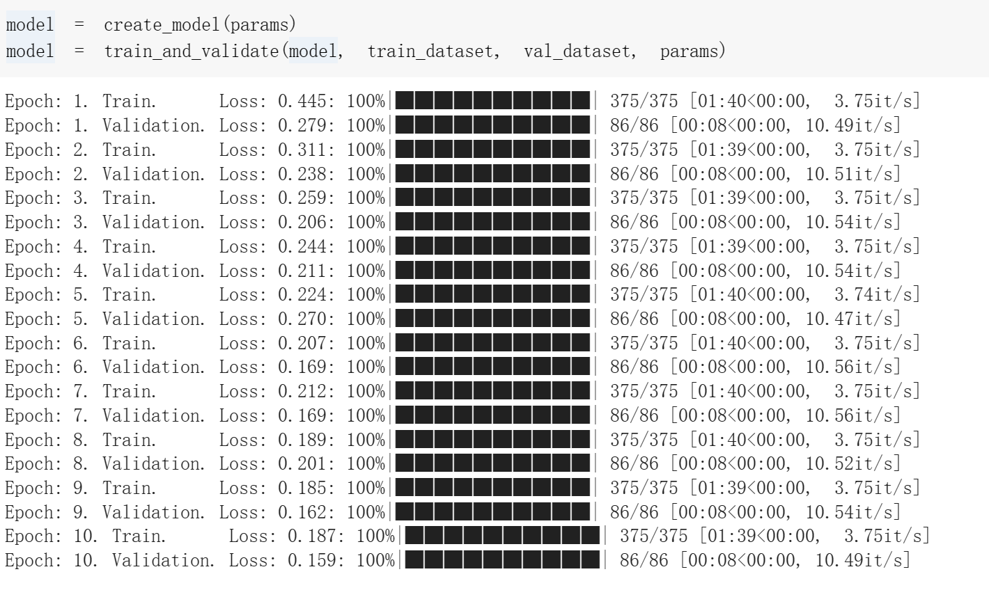
Fig 15. Validation loss of the original UNet11 model

Discussion

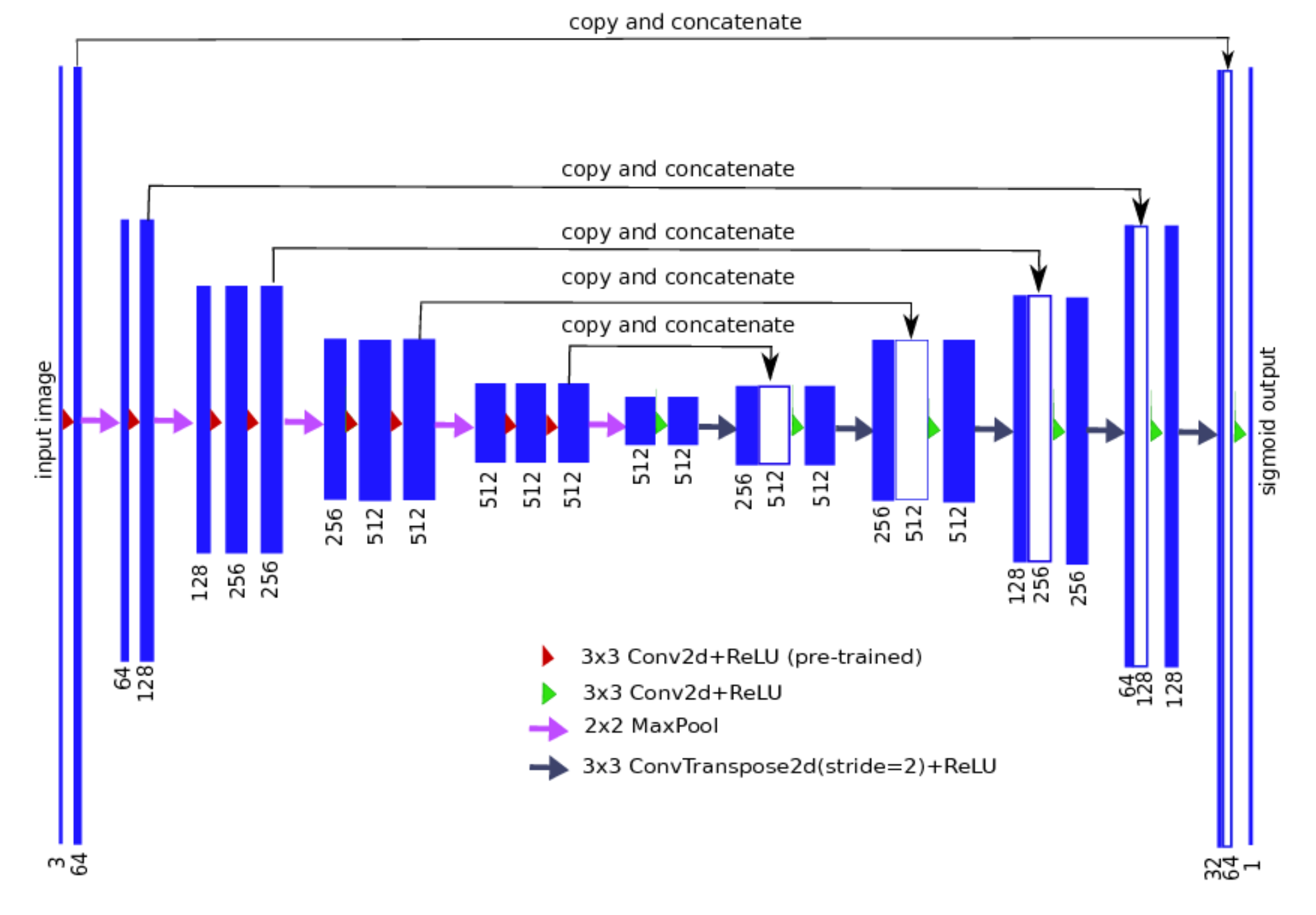
Fig 16. UNet Structure ⁵

We can see that CLIP-based semantic segmentation is able to generate fairly good masks for this dataset. This is a quite surprising result. As can be seen from the above figure⁵, the original model used residual blocks from different convolutional layers to guide the decoder to generate the masks, whereas our model relies on the output of CLIP alone. In addition, from the validation loss, we can see that the final validation loss of our model is comparable to that of the original UNet11 model.

These tell us that CLIP’s feature before the attention pool can be useful in extracting what the objects are as well as where they are. Therefore, CLIP’s feature should be able to perform well on abstracts tasks such as predicting the distance between objects. Since CLIP actually struggle in those tasks, one may suspect that the attention pool layer is to be blamed. We think that modifying the attention pool layer to improve CLIP’s zero-shot performance on abstract tasks may be a good direction for future work, though we do not have additional time to work on it for this project.

Conclusion

We see that the initialization method that we propose solves the problem of few-shot predictors underperforming the zero-shot predictor, though we find that is a more fundamental overfitting problem for the very concept of few-shot learning. For the other problem, that CLIP doesn’t perform well on abstract tasks, the performance of semantic segmentation and generative models based on CLIP seems to suggest that CLIP’s feature before the final attention pool does contain a lot of information, which should be helpful for it in such tasks. This suggests that one may consider adjusting the attention pool layer in future works.

Spotlight Presentation

Click this if the above source doesn’t work.

Reference