Deep Learning-Based Single Image Super-Resolution Techniques
Image super-resolution is a process used to upscale low-resolution images to higher resolution images while preserving texture and semantic data. We will outline how state-of-the art techniques have evolved over the last decade and compare each model to its predecessor. We will also show PyTorch implementations for some of the described models.
Demo
Our final models can be found in the form of interactive Jupyter Notebooks on our related project GitHub repository
Notes:
- The second set of graphs in the video is incorrect. The blog post below contains the correct graphs.
- After the creation of this video, we found a minor error in our SRCNN implementation (placement of ReLU operation). After fixing it, we retrained the model for 50 epochs and achieved a higher PSNR.
- We also trained the GAN for more epochs and witnessed an improvement in perceptual similarity. The loss metrics were similar.
Introduction
Single-Image Super-Resolution (SISR) refers to the process of recovering a high-resolution image from a low-resolution counterpart. This is a classic example of an undetermined inverse problem, as there are multiple possible “solutions” for a given low-resolution image.
 |
|---|
| fig 1. An example of three different image super-resolution models |
In this blog post, we will compare and constrast four super-resolution techniques via: classical methods, sparse coding, deep convolutional neural networks, and generative adversarial models.
Evaluation Metrics
Before diving into the methods of super-resolution, let us first define how we measure the effectiveness of a model.
Peak Signal-to-Noise Ratio
Peak Signal-to-Noise Ratio (PSNR) is a commonly-used metric which takes the ratio between the maximum magnitude of a signal and the magnitude of noise with respect to the signal at its peak clarity. Let us call the ground truth image \(I\) and our super-resolved image \(K\) where both images are of dimension \(h \times w\).
First, we calculate the mean squared error between images (MSE):
\[MSE = \tfrac 1 {h \times w} \sum*{i=0}^{h-1}\sum*{j=0}^{w-1}[I(i,j)-K(i,j)]^2\]Then, PSNR is defined, in decibels, as:
\[\begin{align*} PSNR&=10 \cdot \log_{10} \left(\tfrac{MAX^2_I}{MSE}\right)\\ &= 20 \cdot \log_{10} \left(\tfrac{MAX_I}{\sqrt{MSE}} \right)\\ &= 20 \cdot \log_{10}(MAX_I)-10\cdot \log_{10}(MSE) \end{align*}\]where MAX is the maximum value of a pixel (e.g., for a standard 8-bit image, this would be 255). Note that the formulas above are stated for single-channel images, but are easily generalized to RGB images by simply calculating the average across channels.
Intuitively, a high PSNR implies a better model because it minimizes the MSE between images.
Structural Similarity Index Measure
Structural Similarity Index Measure (SSIM) is a metric that attempts to predict the percieved quality of an image. SSIM is comprised of three sub-comparisons between two samples: luminance, contrast, and structure.
The Structural Similarity Index Measure is then defined as:
\[SSIM(x,y)=l(x,y)^\alpha + c(x,y)^\beta + s(x,y)^\gamma\]for weights, \(\alpha\), \(\beta\), and \(\gamma\) (often set to 1). \(l(x,y)\), \(c(x,y)\), and \(s(x,y)\) defined as:
\[l(x,y) = \tfrac{2\mu_x \mu_y + c_1^2}{\mu_x^2 + \mu_y^2 + c_1^2},\quad c(x,y) = \tfrac{2\sigma_x \sigma_y + c_2^2}{\sigma_x^2 + \sigma_y^2 + c_2^2},\quad s(x,y) = \tfrac{\Sigma_{xy} + c_3^2}{\sigma_x^2\sigma_y^2+ c_3^2}\\\\\]where \(c_i = (k_i \cdot MAX_I)^2\) for some constant \(k_i\).
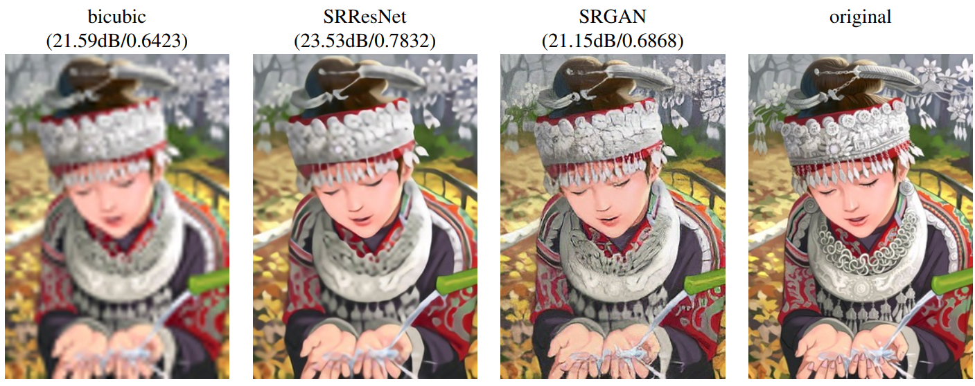
Perceptual Similarity
Although PSNR and SSIM are theoretically sound evaluation metrics, empirical results have shown that they do not effectively capture perceptual similarity. In layman’s terms, a high-resolution image and super-resolution image may both have the same PSNR, but their perceptual quality to the human eye may greatly differ. This is often because error-based metrics such as PSNR do not account for fine textural detail.
 |
|---|
| fig 2. Although the SRResNet model has a higher PSNR, the SRGAN model better preserves textural details in the background. |
Since perceptual similarity is a qualitative property, it is measured through a Mean Opinion Score (MOS) metric. MOS works by essentially averaging the subjective quality of an image across multiple human-answered surveys.
Classical Image Upsampling Techniques
While we will not discuss classical image upsampling techiniques in detail, we will use them as a baseline to compare the results of our models with.
Bicubic Interpolation
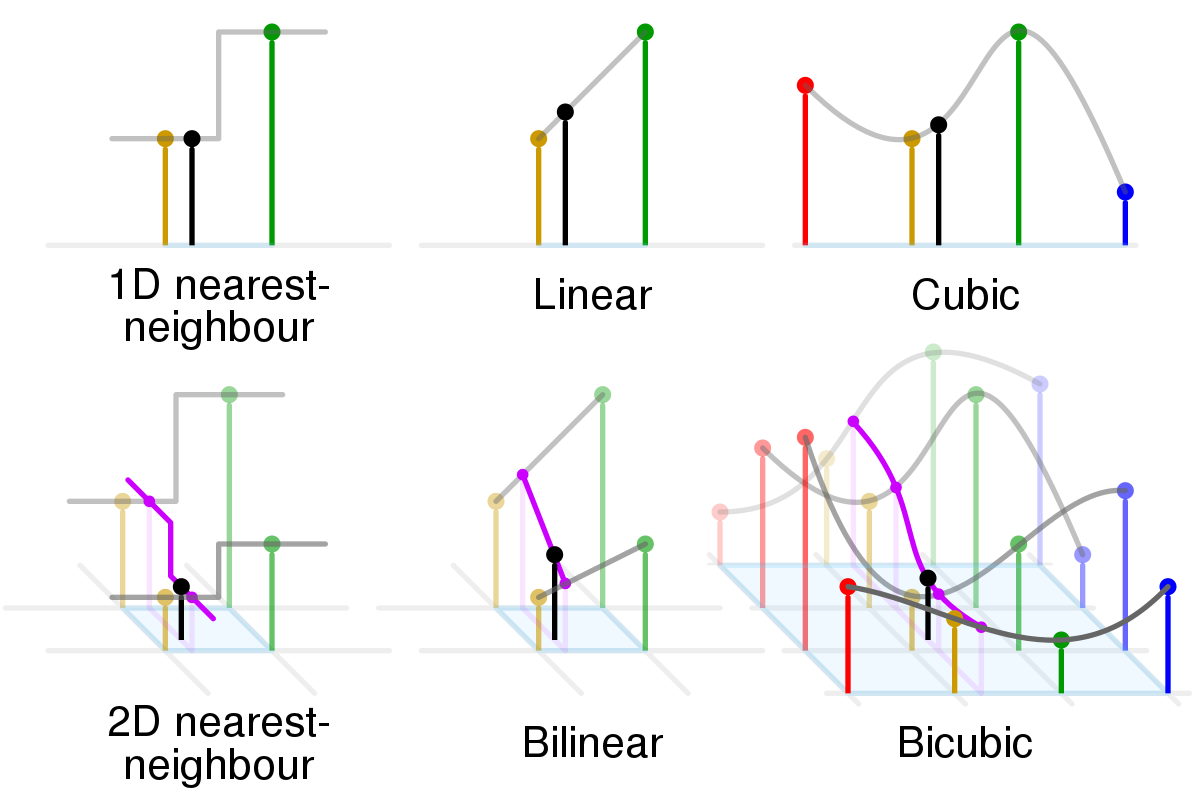 |
|---|
| fig 3. Different interpolation methods where the black dot is the interpolated estimate based on the red, yellow, green, and blue samples. |
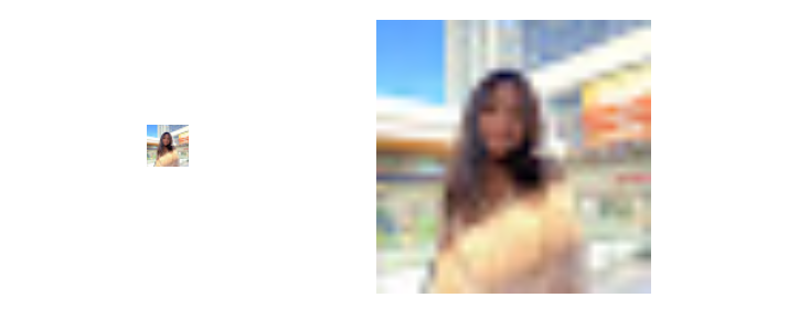
Bicubic interpolation samples 16 in the original low-resolution image for each pixel in the upscaled image. Here’s a real life example where I upsize my profile picture.
 |
|---|
| fig 4. Bicubic interpolation on my profile picture. |
Bicubic interpolation and other similar methods are used widely because they are memory efficient and require comparatively less computational power than deep learning models. However, because there is no learning involved, the super-resolved images do not actually recover any information. For instance, if you’ve ever resized an image on a document as I did above, you’ll know that although you can make the image dimension larger, it will make the image blurry.
Sparse Coding
The sparse coding method is an example-based mathematical method of super-resolution that is an improvement compared to bicubic interpolation because it leverages information provided in training data. Specifically, we discuss Yang et al.’s 2008 sparse coding method.
The essence of this technique is treating the low-resolution image as a downsampled version of its high-resolution counterpart. This was inspired by the idea in signal processing that the original signal can be fully and uniquely recovered from a sampled signal under specific conditions.
Under this assumption, sections of the downsampled image (referred to as patches) can be uniquely mapped to their high-resolution counterpart using a textural dictionary that stores example pairs of low and high resolution image patches.
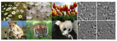
These dictionaries are generated by randomly sampling patches for training images of similar distribution. For example, if we want to upscale animal images, we generate our training dictionary with images that contain fur, skin, and scale textures. For a given category of images, we need only about 100,000 images which is considerably smaller than previous methods. Once patches are generated, we subtract the mean value of each patch as to represent image texture rather than absolute intensity.
 |
|---|
| fig 5. Training images and the patches generated from them. |
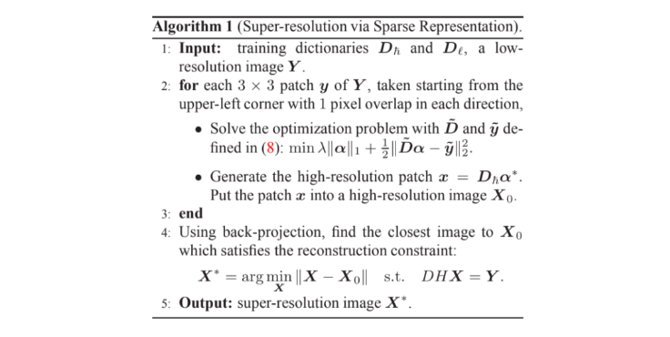
The algorithm of sparse coding super-resolution is as follows: take overlapping patches of the input image, find the sparse coded approximation of the low-resolution patch, map to a high-resolution patch, combine into a locally consistent recovered image by enforcing that the reconstructed patches agree on areas of overlap.
 |
|---|
| fig 6. Formal algorithm of sparse coding super-resolution. |
The uniqueness property of the mapping comes from the linear algebra of sparse matrices. Essentially, because our textural dictionaries are sufficiently large, we can define any low-resolution image as a linear combination of the training patches. This condition is referred to as having an overcomplete basis. Under certain conditions, the sparsest representation (meaning the linear combination using the least patches) is unique—hence the name sparse coding.
Deep CNN-based Super-Resolution
SRCNN
At the start of the millennium, artificial intelligence and deep learning became a quickly exploding field of computer science. Because of the shortcomings of mathematical methods, research on image super-resolution began leveraging this newfound power of deep learning. One of the first pivotal deep learning approaches to image super-resolution was the SRCNN model developed in 2015.
Moving Forward from Sparce Coding
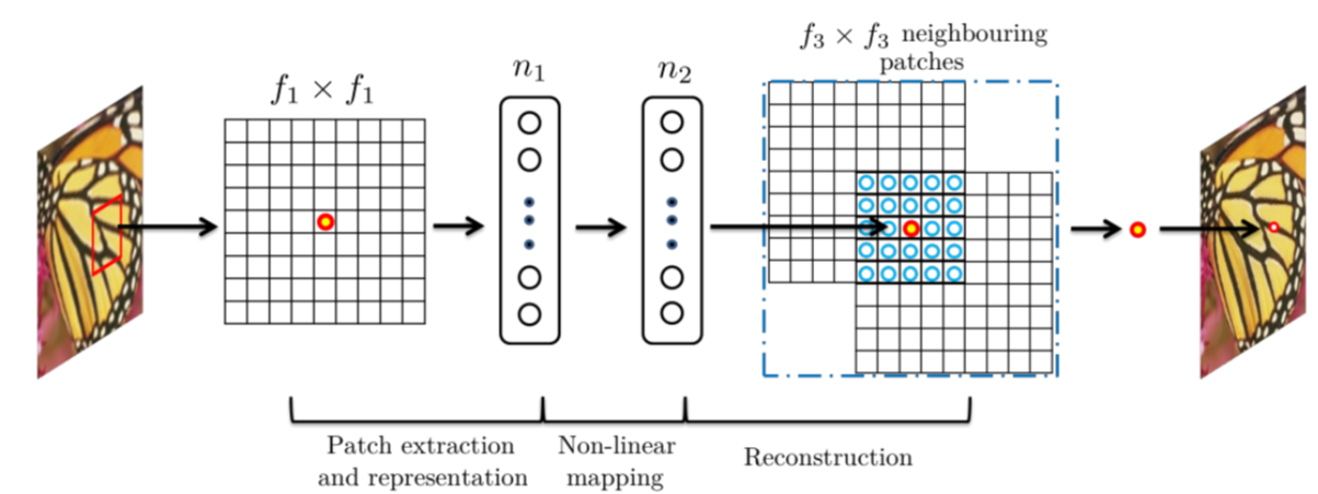
The SRCNN is essentially a deep convolutional neural network representation of the aforementioned sparse coding pipeline. Each step of the SC pipeline can be implicitly represented as a hidden layer of the CNN.
Patch Extraction and Representation
In sparse coding, this operation extracts overlapping patches from the low-resolution image and represents them as a sparse linear combination of the basis.
With a neural net, this is equivalent to convolving the image with a filter representing the basis. SRCNN convolves the image with multiple filters each of which represents a basis. The selection of these bases is folded into the optimization of the network instead of being hand-selected as it is in sparse coding. This results in a \(n_1\)-dimensional feature for each patch.
The intuition behind having multiple bases stems from wanting a generalizable model. The sparse coding algorithm generates a dictionary based on training examples of similar images (nature images for flowers, furtextures for animals, etc.). In contrast, because a neural net learns the optimal weights, it will implicitly choose the bases that best fit with the training data.
Non-linear Mapping
In sparse coding, this operation maps each low-resolution patch to a high-resolution patch.
With a neural net, we want to map each \(n_1\)-dimensional feature to a \(n_2\)-dimensional feature representing the high-resolution patch. This is equivalent to applying \(n_1\) filters of size \(1 \times 1\).
Reconstruction
In sparse coding, this operation aggregates all the high-resolution patches to generate the final reconstructed image.
We can think of this as “averaging” the overlapping patches which corresponds to an averaging filter.
 |
|---|
| fig 7. Sparse coding as a CNN. |
Since Yang et. al’s 2008 sparse coding algorithm, many changes have been proposed to improve the speed and accuracy of mapping low-resolution patches to their high-resolution counterparts. However, the dictionary generation and patch aggregation processes are considered pre/post-processing and thus have not been subject to the same optimization. The key advantage of using a CNN for the process is that because all steps of the pipeline are implicitly embedded into the network, they are equally subject to learning as the model finds the optimal weights.
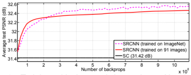
Furthermore, the sparse coding algorithm is an iterative algorithm, taking one pass per patch of the input image. In contrast, SRCNN is a fully feed-forward neural net and it reconstructs the image in a single pass. Below, we can see that SRCNN bypasses the sparse coding algorithm in just a few iterations.
 |
|---|
| fig 8. PSNR of SRCNN. |
Model Architecture
SRCNN generates training samples by first cropping HR images by randomly. A low resolution counterpart is then created by first applying a Gaussian kernel, then applying bicubic downsampling and upsampling to return the LR image to the original size.
SRCNN uses MSE as the loss function between the reconstructed images and the corresponding ground truth images which is minimized using stochastic gradient descent with momentum.
The weights are initialized from a Gaussian distribution with zero mean. The learning rate is 10-4 for the first two layers and 10-5 for the last layer.
The base setting for parameters is \(f_1=9\), \(f_2=1\), \(f_3=5\), \(n_1=64\), and \(n_2=32\) where \(f_i\) is the size of the \(i\)th filter and \(n_i\) is as defined above.
During training, to avoid issues with black borders, no padding is used. Thus, the network produces a slightly smaller output. The MSE loss is evaluated only by the pixels that overlap. The network also contains no pooling or fully-connected layer.
Empirical results show that a deeper structure does not necessarily lead to better results, which is not the case for the image classification models we studied in class. However, a larger filter size was found to improve performance.
Color Images
Up until now, we have not discussed how to deal with multi-channel images in our SR algorithms. The conventional approach to super-resolve color images is to first transform the images into the YCbCr space. The Y channel is the luminance, while the Cb and Cr channels are the blue-difference and red-difference channels, respectively. Then, we train the proposed algorithm on only the Y channel while the Cb and Cr channels are upscaled through bicubic interpolation.
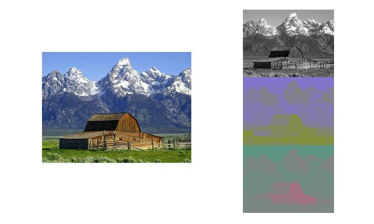 |
|---|
| fig 9. An image of a mountain separated into its YCbCr channels. |
Generative Adversarial Network-based Super-Resolution
SRGAN
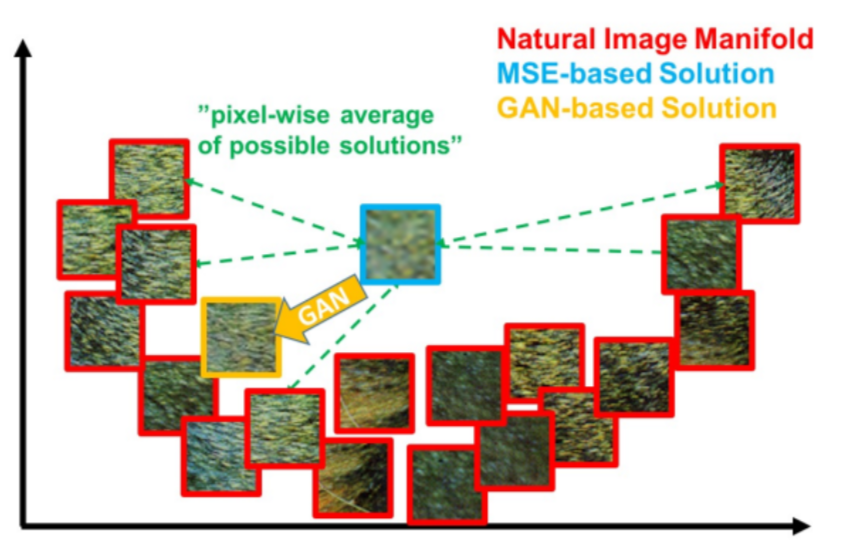
Although deep convolutional neural networks were a breakthrough in the field of image super-resolution, a key challenge they faced was that they were unable to recover fine textural details. In 2016, a generative adversarial model for super-resolution called SRGAN was proposed that showed significant empirical improvement in perceptual similarity when compared with SRCNN.
 |
|---|
| fig 11. Patches from the natural image manifold (red) and super-resolved patches obtained with MSE (blue) and GAN (orange). The MSE-based solution appears overly smooth due to the pixel-wise average of possible solutions in the pixel space, while GAN drives the reconstruction towards the natural image manifold producing perceptually more convincing solution. |
Moving Forward from Convolutional Neural Networks
Generative adversarial models work by simultaneously training two networks: a generator that is trained to generate the best possible solution and a discriminator which is trained to differentiate between generated solutions and ground truth. The two networks learn jointly in a minimax game as they try to fulfill opposite goals.
One of the most important improvements with SRGAN is the addition of a “perceptural loss” for the generator. Recall our earlier discussion of loss functions, where we noted the difference between perceptual similarity and pixel similarity. SRGAN allows for better recovery of textural detail by defining a loss function which prioritizes perceptual similarity over pixel similarity.
The pereptual loss function is defined as weighted sum of a content loss and the adversarial loss.
- Content Loss (VGG Loss): Instead of using a pixel-based MSE loss, we calculate the loss based on the Euclidian distance between feature maps produced by VGG-16 of the ground truth image and the super-resolved image. Thus, for the feature map after the \(j\)th convolution and before the \(i\)th max-pooling layer in VGG-16 (\(\phi_{i,j}\)), the content loss is defined as:
- Adversarial Loss: We want to maximize the discriminator network’s perceived probability that the reconstructed image is a natural image. This encourages perceptually superior solutions because we prioritize similarity to natural images instead of only evaluating MSE loss. Adversarial loss is defined as:
Ledig et al. speculate that this method of evaluation improves recovery of textural detail because feature maps of deeper layers focus purely on the content while leaving the adversarial loss to manage textural details which are the main difference between CNN-produced super-resolved images and natural images. However, this loss function may not be ideal for all applications. For example, hallucination of finer detail may be less suited for medical or surveillance fields.
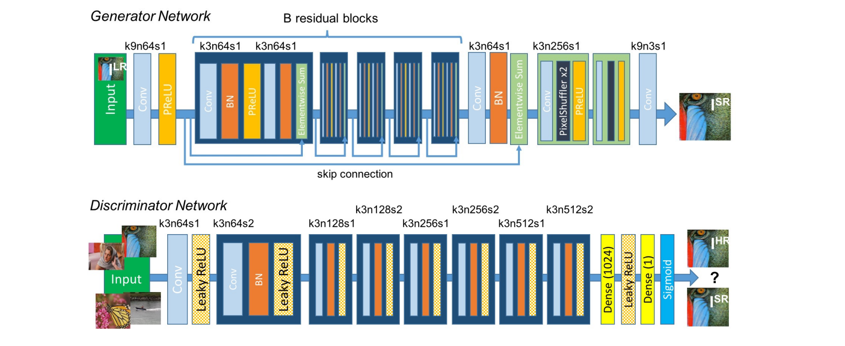
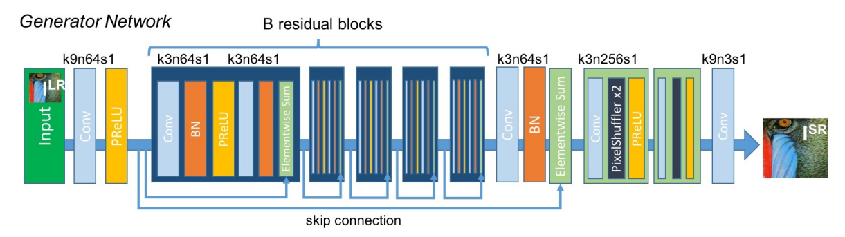
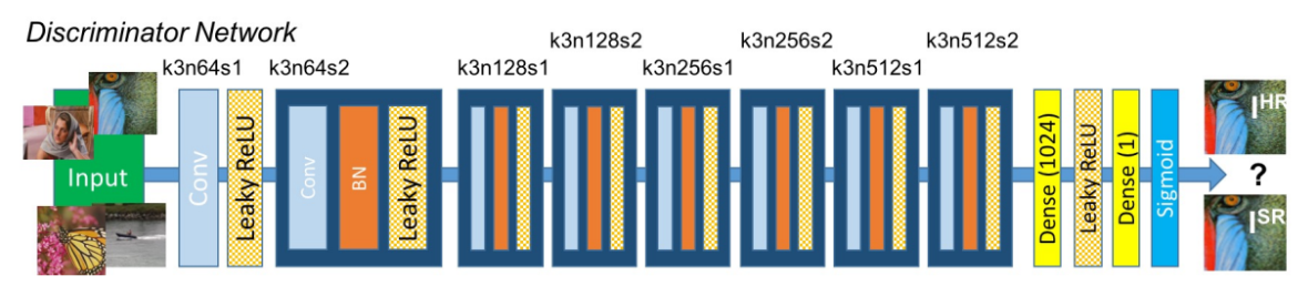
Model Architecture
The generator network is a residual neural network that uses two convolutional layers with small \(3 \times 3\) kernels and 64 feature maps followed by batch-normalization layers and PReLU as the activation function.
The discriminator network is a feed-forward network that contains eight convolutional layers with an increasing number of \(3 \times 3\) filter kernels, increasing by a factor of 2 from 64 to 512 kernels similar to the VGG-19 network. Strided convolutions are used to reduce the image resolution each time the number of features is doubled. The resulting 512 feature maps are followed by two fully-connected layers and a final sigmoid activation. We use LeakyReLU as the activation (\(\alpha = 0.2\)) and avoid max-pooling.
 |
|---|
| fig 12. Model architecture for SRGAN discriminator and generator. |
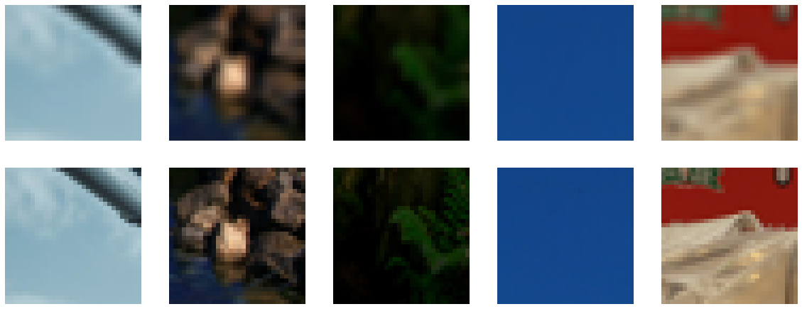
Real-ESRGAN
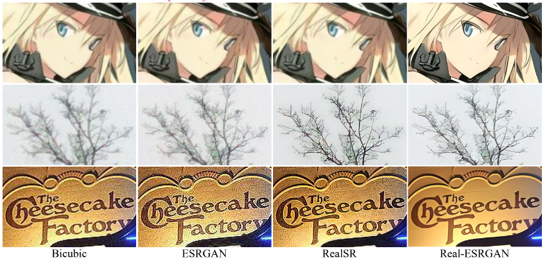
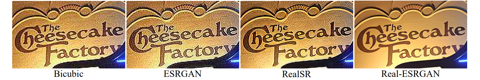
After SRGAN, an improved version called ESRGAN (Enhanced SRGAN) was released in 2018 with some network tweaks. However, the current state-of-the-art model in image super-resolution is Real-ESRGAN, an improvement upon ESRGAN that was released in 2021. The key difference is that Real-ESRGAN is trained on purely synthetic data that is generated through a multi-step degradation process designed to simulate real-life degradations. In contrast, ESRGAN simply applies a Gaussian filter followed by a bicubic downsampling operation. This method removes artifacts that were previously common when super-resolving common real-world images.
 |
|---|
| fig 13. Comparisons of bicubic-upsampled, ESRGAN, RealSR, and Real-ESRGAN results on real-life images. The Real-ESRGAN model trained with pure synthetic data is capable of enhancing details while removing artifacts for common real-world images. |
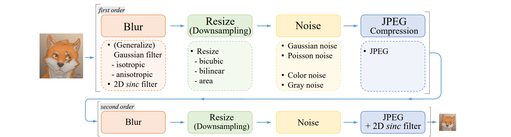
Super-Resolution for Multiple Degredations
Real-ESRGAN uses a high-order degradation model which means that image degradations are modeled with several repeated degradation process. The following are the steps in a single block of the degradation process
- Blur: Apply a Gaussian blur filter (same as SRGAN)
- Noise: Gaussian or Poisson noise filter is added independently to each RGB color channel. Gray noise is also synthesized by adding the same noise to all channels.
- Downsampling: Apply random resize operation chosen from nearest-neighbor interpolation, area resize, bilinear interpolation, and bicubic interpolation.
- JPEG Compression: JPEG compression is a echnique of lossy compression for images. It first converts images into the YCbCr color and then downsamples the Cb and Cr channels. This often results in image artifacts.
- Sinc filters: A sinc filter is used to simulate common ringing and overshoot artifacts in images.
Empirically, this allows for super-resolution with respect to multiple types of image degredations. For example, images which have been compressed multiple times (perhaps by being repeatedly uploaded to different social media sites) can be super-resolved whereas SRGAN and SRCNN trained with only bicubic degreadation cannot.
 |
|---|
| fig 14. Overview of the pure synthetic data generation adopted in Real-ESRGAN. It utilizes a second-order degradation process to model more practical degradations, where each degradation process adopts the classical degradation model. |
Model Implementations in PyTorch
For our implementation, we chose to recreate and compare SRCNN and SRGAN using PyTorch. Our final models can be found in the form of interactive Jupyter Notebooks on our related project GitHub repository. Final trained weights for both models can also be found there.
Dataset Preparation
For simplicity, instead of the traditional train-test-val sets, we used a single dataset for the training and testing. Specifically, we used a dataset designed for super-resolution tasks downloade from Kaggle. The training was performed on randomly selected patches of of the images and the testing was performed on the full images.
 |
|---|
| fig 15. Examples of images in the training set. |
Evaluation Metrics
Before training any models, we must define our evaluation metrics as shown below.
def mse(pred, label):
    mse_val = torch.mean((pred - label)**2)
    return mse_val

def psnr(pred, label):
    mse_val = mse(pred, label)
    return 10 * torch.log10(1 / mse_val)

def ssim(pred, label):
    return structural_similarity_index_measure(pred, label)
SRCNN Implementation
Below is our PyTorch implementation of SRCNN. As described, the model is an extremely simple convolutional network, with only three layers. Each layer corresponds to a different step of the sparse coding pipeline as described above.
class SRCNN(nn.Module):
    def __init__(self):
        super(SRCNN, self).__init__()
        self.features = nn.Sequential(
            nn.Conv2d(3,  64, kernel_size=9, stride=1, padding=9 // 2),
            nn.Conv2d(64, 32, kernel_size=5, stride=1, padding=5 // 2),
            nn.Conv2d(32, 3,  kernel_size=5, stride=1, padding=5 // 2),
            nn.ReLU(True),
        )

    def forward(self, x):
        x = self.features(x)
        return x
Deviations From the Paper
Unlike in the paper, we padded each layer such that the output resolution remained the same. This is done as we found that the edge artifacts weren’t very noticable after a small number of training epochs. We also trained on all channels in RGB color space (as opposed to training on the Y channel in YCrBr color space as in the paper).
Additionally, we used the Adam optimizer to optimize the loss with standard values for \(\beta_1\) and \(\beta_2\). We also used patch sizes of \(32 \times 32\).
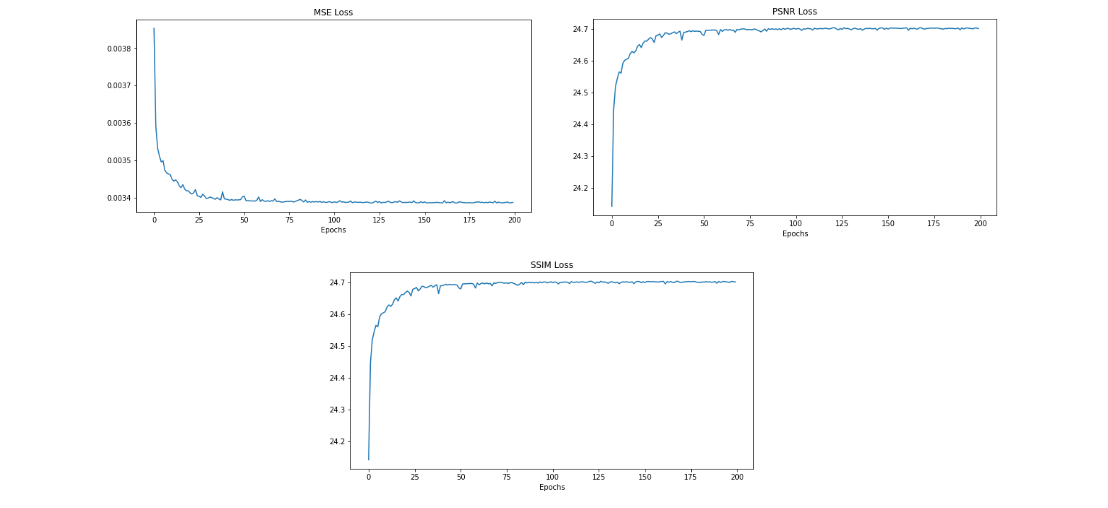
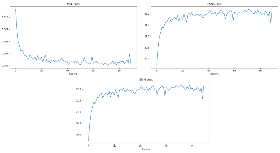
SRCNN Training
As described in the paper, we train by minimizing MSE loss, but we also record PSNR and SSIM losses during the training process. Note that the learning rate is different for each layer and that we save the weights after training so that we can run the test phase without retraining each time.
Below you see the loss for each evaluation metric. Something we observed is that the loss plateaus earlier than 200 epochs so it may not have been necessary to train this long.
 |
|---|
| fig 16. MSE/PSNR/SSIM loss from SRCNN training. |
SRCNN Results
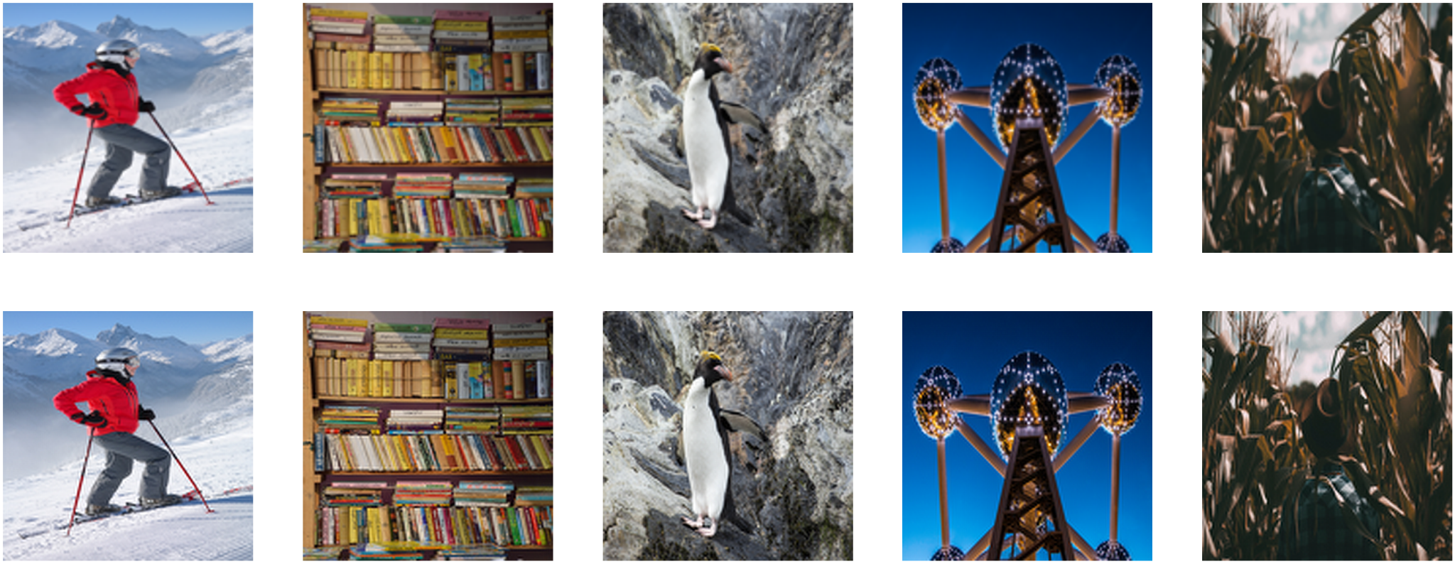 |
|---|
| fig 17. Super-resolution results from SRCNN. |
 |
|---|
| fig 18. Zooming into a particular image. |
As you can see, such a simple CNN delivers powerful results on the above images.
SRGAN Implementation
Implementing the SRGAN architecture was a much more challenging feat than SRCNN. SRGAN, like other GAN-based models, is comprised of two major parts: the generator and discriminator.
Generator Implementation
 |
|---|
| fig 19. SRGAN generator architecture. |
Below is our PyTorch impelementation of the SRGAN generator (SRResNet). It consists of 16 residual block encoder along with a decoder.
class SRResNet(nn.Module):
    def __init__(self, res_depth=16, upsample_scale=4):
        super(SRResNet, self).__init__()
        self.conv = nn.Sequential(
            nn.Conv2d(3, 64, kernel_size=9, stride=1, padding=9 // 2),
            nn.PReLU(),
        )
        self.encoder = nn.Sequential(
            ResidualBlock(64, res_depth),
            nn.Conv2d(64, 64, kernel_size=3, stride=1, padding=1),
            nn.BatchNorm2d(64),
        )
        self.decoder = nn.Sequential(
            UpsampleBlock(64, upsample_scale),
            nn.Conv2d(64, 3, kernel_size=9, stride=1, padding=9 // 2)
        )

    def forward(self, x):
        x = self.conv(x)
        x = self.encoder(x) + x
        x = self.decoder(x)
        return x
Residual Block
class ResidualBlock(nn.Module):
    def __init__(self, channels, depth):
        super(ResidualBlock, self).__init__()
        self.residual_blocks = nn.ModuleList([nn.Sequential(
            nn.Conv2d(channels, channels, kernel_size=3, stride=1, padding=1),
            nn.BatchNorm2d(channels),
            nn.PReLU(),
            nn.Conv2d(channels, channels, kernel_size=3, stride=1, padding=1),
            nn.BatchNorm2d(channels),
        ) for _ in range(depth)])

    def forward(self, x):
        for residual_block in self.residual_blocks:
            x = residual_block(x) + x
        return x
Upsample Block
class UpsampleBlock(nn.Module):
    def __init__(self, in_channels, upsample_scale):
        super(UpsampleBlock, self).__init__()
        factor = 2 if upsample_scale % 2 == 0 else upsample_scale
        out_channels = in_channels * factor**2
        self.upsample_blocks = nn.ModuleList([nn.Sequential(
            nn.Conv2d(in_channels, out_channels, 3, stride=1, padding=1),
            nn.PixelShuffle(factor),
            nn.PReLU(),
        ) for _ in range(upsample_scale // 2)])

    def forward(self, x):
        for upsample_block in self.upsample_blocks:
            x = upsample_block(x)
        return x
Discriminator Architecture
 |
|---|
| fig 19. SRGAN generator architecture. |
Below is our PyTorch implementation of the SRGAN discriminator. The discriminator is a standard convolutional neural netowrk consisting of many blocks which reduce the input size, but increase the number of filters.
Note that due to the hardcoded input size for the first fully-connected lyaer of the classifier, the input image size of the discriminator must be \(96 \times 96\)
class DiscriminatorBlock(nn.Module):
    def __init__(self, in_channels, out_channels):
        super(DiscriminatorBlock, self).__init__()
        stride = 2 if in_channels == out_channels else 1
        self.features = nn.Sequential(
            nn.Conv2d(in_channels, out_channels, 3, stride=stride, padding=1),
            nn.BatchNorm2d(out_channels),
            nn.LeakyReLU(0.2, inplace=True),
        )

    def forward(self, x):
        x = self.features(x)
        return x


class Discriminator(nn.Module):
    def __init__(self):
        super(Discriminator, self).__init__()
        self.conv = nn.Conv2d(3, 64, kernel_size=3, stride=1, padding=1)
        self.features = nn.Sequential(
            DiscriminatorBlock(64,  64),
            DiscriminatorBlock(64,  128),
            DiscriminatorBlock(128, 128),
            DiscriminatorBlock(128, 256),
            DiscriminatorBlock(256, 256),
            DiscriminatorBlock(256, 512),
            DiscriminatorBlock(512, 512),
        )
        self.classifier = nn.Sequential(
            nn.Linear(18432, 1024),
            nn.LeakyReLU(0.2),
            nn.Linear(1024, 1),
        )
        self.lrelu = nn.LeakyReLU(0.2)

    def forward(self, x):
        batch_size = x.shape[0]

        x = self.lrelu(self.conv(x))
        x = self.features(x)
        x = x.flatten(1)
        x = self.classifier(x)
        return torch.sigmoid(x.view(batch_size))
Loss Functions
To define our loss functions for the generator and discriminator, we first need three “building block” losses; the combination of these losses allows for multiple sub-tasks to be learned at once.
- Pixel Loss (MSE)
- Content Loss (VGG)
- Adversarial Loss (BCE)
For the content loss (VGG loss), we define a feature exraction module which extracts the feature map from the features layer of the torchvision.models.vgg16 model. The forward pass of the module extracts the features from the input images and calculates the MSE between the features:
class ContentLoss(nn.Module):
    def __init__(self, device):
        super(ContentLoss, self).__init__()
        vgg19 = models.vgg19(pretrained=True).to(device)
        for param in vgg19.parameters():
            param.requires_grad = False

        self.features = nn.Sequential(*list(vgg19.children())[0][:36])

    def forward(self, inputs_real, inputs_fake):
        real_features = self.features(inputs_real)
        fake_features = self.features(inputs_fake)

        return F.mse_loss(real_features, fake_features)
Our generator and discriminator losses used for training are then defined as such:
generator_loss =
     1e-0 * pixel_criterion(inputs_fake, inputs_real) +
     6e-3 * content_criterion(inputs_fake, inputs_real) +
     1e-3 * adversarial_criterion(fake_prob.detach(), labels_real)

discriminator_loss =
     adversarial_criterion(real_prob, labels_real) +
     adversarial_criterion(fake_prob, labels_fake)
SRGAN Training
There are two steps to train SRGAN: A SRResNet (generator) pretraining process such that the generator of SRGAN can be initialized with weights that avoid undesired local minima when training, and a adversarial minimax training process between the generator and discriminator. We pretrained our SRResNet for 90 epochs and trained the SRGAN model for 20 epochs.
Below, we see the training losses from the pre-training process.
 |
|---|
| fig 20. MSE/PSNR/SSIM loss from SRGAN training. |
Deviations From the Paper
Unlike in the paper, our discriminator implementation has a Sigmoid operation at the end of the forward pass to output the un-normalized probabilities of the discriminator. This allowed us to use the nn.BCELoss() from the PyTorch library.
Additionally, the paper describes the addition of a very-lightly weighted Total Variation (TV) loss when using earlier feature maps of VGG-19 which we omitted from our training process. Additionally, no learning rate scheduling was used during our training process (\(\eta = 10^{-5}\)).
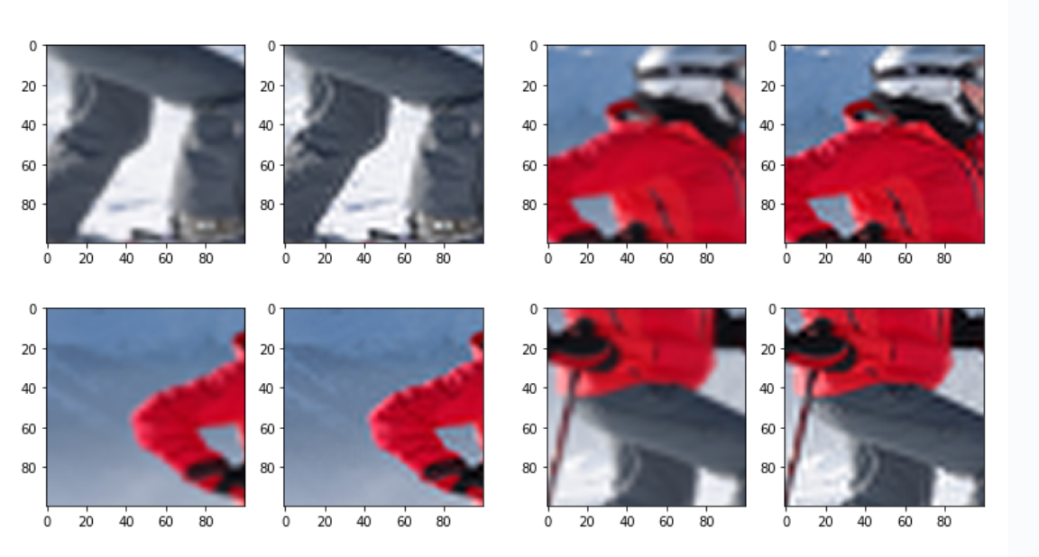
SRGAN Results
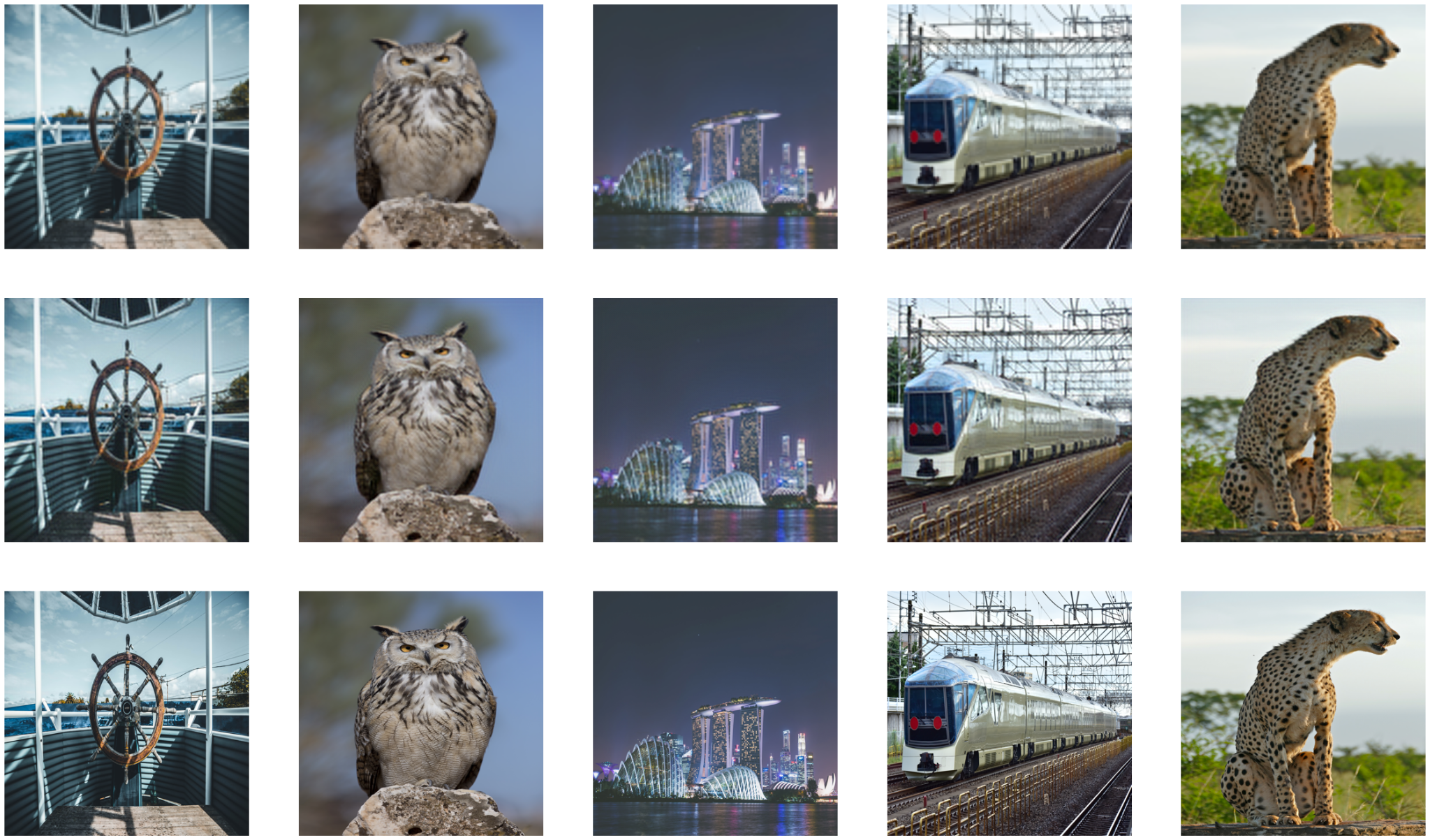 |
|---|
| fig 21. Super-resolution results from SRGAN. The first row is the original image, the second row is the super-resolved image, and the third row is the original high-resolution image. |
Comparison
Ultimately, SRCNN achieved a PSNR of 24.7 dB on the test set while SRGAN achieved 22.1 dB. The PSNR before any super-resolution was performed is approximately 23.9.
These results seem counterintuitive initially because it seems like SRGAN showed no improvement. A partial reason for this is likely that we did not have the time or credits to train the model for longer. It took about 5 hours hours to train the GAN for 20 epochs (not including the pre-training process), which was much slower than SRCNN because of the increased complexity.
However, as we discussed above, we must note that PSNR and other MSE-based evaluation metrics do not capture perceptual similarity which was prioritized in the implementation of SRGAN. In the source paper, SRGAN showed a very minimal increase in PSNR compared to the bicubic baseline after training. Furthermore, both PSNR and SSIM decreased while training the GAN after the pre-training process. However, the images themselves seemed more realistic to the human eye. Our model shows similar results and preserves textural details better than our implementation of SRCNN.
Conclusion
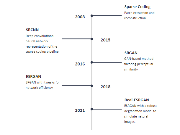 |
|---|
| fig 15. Timeline of SR methods. |
So far in our discussion of the evolution of methods for single image super-resolution, we have covered four key models: sparse coding, SRCNN, SRGAN, and Real-ESRGAN (the current state-of-the-art). We have gone on to recreate the SRCNN and SRGAN models. Of course, there are other models in the field that we have not been able to cover in detail today. One notable mention is the transformer based model, Efficient Super-Resolution Transformer (ESRT) released last year. Although there has been rapid improvement in the field of super-resolution, there are still many challenges to overcome. Current research is focused on expanding single image super-resolution to video resolution, reducing the amount of data needed to simulate real-world degradation processes, and fine-tuning models for specific SR tasks such as face reconstruction.
References
[1] Jianchao Yang, J. Wright, T. Huang and Yi Ma, “Image super-resolution as sparse representation of raw image patches,” 2008 IEEE Conference on Computer Vision and Pattern Recognition, Anchorage, AK, USA, 2008, pp. 1-8, doi: 10.1109/CVPR.2008.4587647.
[2] Dong, Chao, et al. “Image Super-Resolution Using Deep Convolutional Networks.” IEEE Transactions on Pattern Analysis and Machine Intelligence. 2014.
[3] Ledig, Christian, et al. “Photo-Realistic Single Image Super-Resolution Using a Generative Adversarial Network.” Proceedings of the IEEE conference on computer vision and pattern recognition. 2017.
[4] Wang, X. et al. (2019). “ESRGAN: Enhanced Super-Resolution Generative Adversarial Networks.” In: Leal-Taixé, L., Roth, S. (eds) Computer Vision – ECCV 2018 Workshops. ECCV 2018. Lecture Notes in Computer Science(), vol 11133. Springer, Cham. https://doi.org/10.1007/978-3-030-11021-5_5
[5] X. Wang, L. Xie, C. Dong and Y. Shan, “Real-ESRGAN: Training Real-World Blind Super-Resolution with Pure Synthetic Data,” 2021 IEEE/CVF International Conference on Computer Vision Workshops (ICCVW), Montreal, BC, Canada, 2021, pp. 1905-1914, doi: 10.1109/ICCVW54120.2021.00217.