Galaxy Detection/Classification with Computer Vision
In this blog, I will share my experience in using a machine learning model (based on YOLO) that detects and classifies galaxies from public datasets from the Sloan Digital Sky Survey (SDSS) and Galaxy Zoo while taking CS 188: Deep Learning for Computer Vision at UCLA.
1. Introduction
Astronomical datasets are constantly increasing in size and complexity. The modern generation of integral field units (IFUs) are generating about 60 GB of data per night while imaging instruments are generating 300 GB of data per night. In particular, the James Webb Space Telescope produces and transmits about 57 GB of data using the Deep Space Network (DSN) and the Large Synoptic Survey Telescope (LSST, now called Vera C. Rubin Observatory) which is under construction in Chile expected to start full operations in 2024. With a wide 9.6 square degree field of view 3.2 Gigapixel camera, LSST will generate about 20 TB of data per night (González et al). Although these astronomical data include a lot more information than intensities measured with specific filters (igr band filters, RBVRI broadband filters), as the size of data produced everyday is increasing over time, deep learning algorithms in computer vision may help researchers to identify key targets to perform more in-depth, conventional analyses.
2. Data Exploration
2-1. SDSS
The Sloan Digital Sky Survey (SDSS), is a massive astronomical survey which was conducted from 2000 to 2008 which collected more than 3 million astronomical objects (stars, galaxies, and quasars) from over 35% of the sky with a 2.5 meter telescope at Apache Point Observatory in New Mexico, United States. Some of the most important discoveries from the SDSS are 1) discovering and characterizing dark energy, 2) understanding the large-scale structure of the Universe through the distribution of galaxies and the presence of cosmic voids, clusters, and filaments.
2-2. Galaxy Zoo
https://www.kaggle.com/competitions/galaxy-zoo-the-galaxy-challenge/data
The Galaxy Zoo (Lintott et al) is one of the most successful citizen project in astronomy, where hundreds of thousands of volunteers classified images of nearly 900,000 galaxies obtained from the SDSS survey by answering questions about their characteristics (Figure 1)
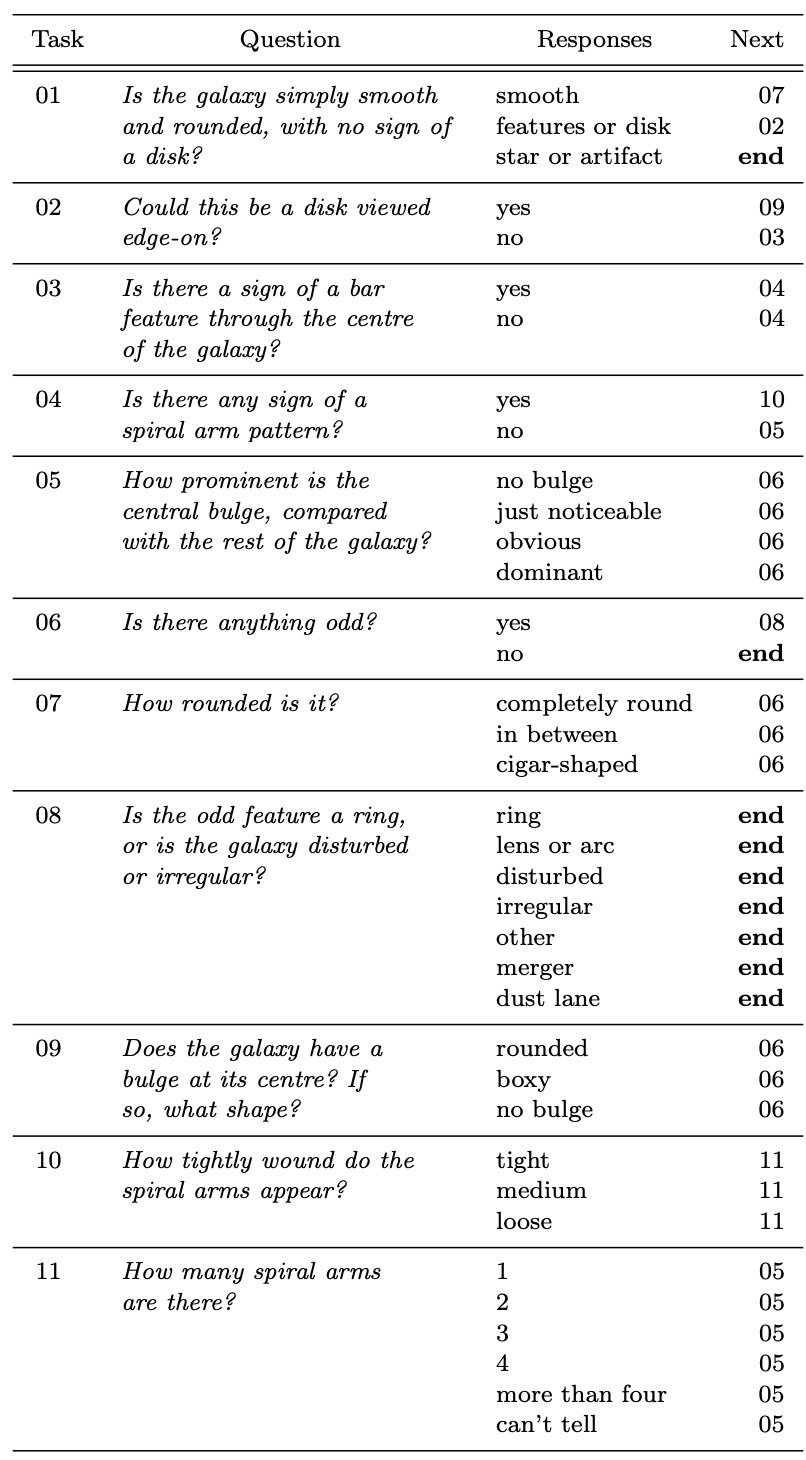
[Figure 1] Decision Tree used to classify galaxies in Galaxy Zoo project.
2-2-1. Labels
- Each galaxy has a matching entry in a separate csv file where each column value represents the ratio of how volunteers (Galaxy Zoo) responded to questions to the decision tree (Figure 1).
| index | GalaxyID | Class1.1 | Class1.2 | Class1.3 | Class2.1 | Class2.2 | Class3.1 | Class3.2 | Class4.1 | Class4.2 |
|---|---|---|---|---|---|---|---|---|---|---|
| 0 | 100008 | 0.383147 | 0.616853 | 0.0 | 0.0 | 0.616853 | 0.038452149 | 0.578400851 | 0.418397819 | 0.198455181 |
| 1 | 100023 | 0.327001 | 0.663777 | 0.009222 | 0.031178269 | 0.632598731 | 0.467369636 | 0.165229095 | 0.591327989 | 0.041270741 |
| 2 | 100053 | 0.765717 | 0.177352 | 0.056931 | 0.0 | 0.177352 | 0.0 | 0.177352 | 0.0 | 0.177352 |
| 3 | 100078 | 0.693377 | 0.238564 | 0.068059 | 0.0 | 0.238564 | 0.109493481 | 0.129070519 | 0.189098232 | 0.049465768 |
| 4 | 100090 | 0.933839 | 0.0 | 0.066161 | 0.0 | 0.0 | 0.0 | 0.0 | 0.0 | 0.0 |
| Class5.1 | Class5.2 | Class5.3 | Class5.4 | Class6.1 | Class6.2 | Class7.1 | Class7.2 | Class7.3 | Class8.1 |
|---|---|---|---|---|---|---|---|---|---|
| 0.0 | 0.104752126 | 0.512100874 | 0.0 | 0.054453 | 0.945547 | 0.201462524 | 0.181684476 | 0.0 | 0.0 |
| 0.0 | 0.236781072 | 0.160940708 | 0.23487695 | 0.189149 | 0.810851 | 0.0 | 0.135081824 | 0.191919176 | 0.0 |
| 0.0 | 0.11778975 | 0.05956225 | 0.0 | 0.0 | 1.0 | 0.0 | 0.74186415 | 0.02385285 | 0.0 |
| 0.0 | 0.0 | 0.113284024 | 0.125279976 | 0.320398 | 0.679602 | 0.408599439 | 0.284777561 | 0.0 | 0.0 |
| 0.0 | 0.0 | 0.0 | 0.0 | 0.029383 | 0.970617 | 0.494587282 | 0.439251718 | 0.0 | 0.0 |
[Table 1] Examples of how volunteers classified Galaxies for GalaxyZoo Project.
2-2-2. Galaxy Images
Some of the images in the dataset look like the figure below.
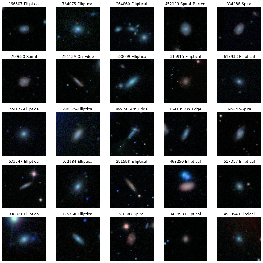
[Figure 2] Galaxies in the Galaxy Zoo Dataset. Each image is labeled with its Galaxy-ID and Galaxy type classified by the volunteers
2-3. SDSS Data
Instead of using cropped images of single galaxies shown above, González et al. used a Python astroquery package to fetch about 20000 field images in FITS format (each with multiple galaxies per single image) from the SDSS database. However, the images fetched from the SDSS are not in a normal RGB format (YOLO method is designed to work with 3-channel color images). Instead, we have access to multiple images of the same field taken with different optical filters. Here, González et al. used three images, each taken with g, r, i band filters. (g-band filter transmits light in the green portion of the spectrum; 400-550 nm, r-band filter transmits light in the red portion of the spectrum; 550-700 nm, and i-band filter transmits light in the near-infrared portion of the spectrum; 700-850 nm). Below are the screenshots of the three FITS images of the same field loaded onto SAOImage DS9, a popular astronomical viewer and analysis tool.

[Figure 3-1] g-band image. g-band filter transmits light in wavelength range 400-550 nm
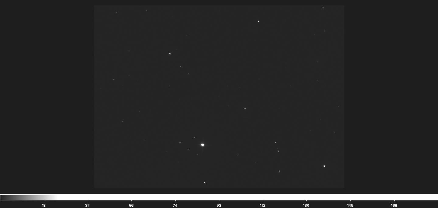
[Figure 3-2] r-band image. r-band filter transmits light in wavelength range 550-700 nm
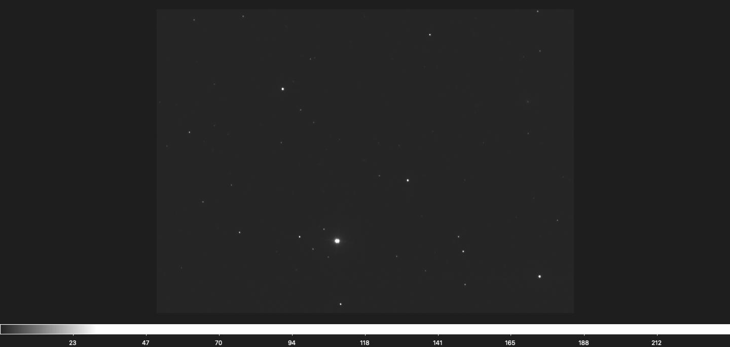
[Figure 3-3] i-band image. i-band filter transmits light in wavelength range 700-850 nm
2-3-1. Lupton Method
Instead of using grayscale images shown above, González et al. used Lupton et al. (2004) as standard conversion method from FITS in igr bands to RGB image which is provided with Astropy, an open-source Python library with a wide range of tools and functions for astronomical data. The basic algorithm of Lupton method follows 4 simple steps.
1) Convert each FITS image to a grayscale image, also considering any appropriate scaling or stretching that may be necessary to ensure that the data values fall within the dynamic range of the output image.
2) Assign each grayscale image to a color channel, with the red channel assigned to the longest-wavelength filter (in this case, i-band filter), the green channel assigned to the intermediate-wavelength filter (r-band filter), and the blue channel assigned to the shortest-wavelength filter (g-band filter).
3) Apply a scaling factor to each color channel to adjust the relative brightness of each channel with
   red = (red - gray_min) / (red_max - gray_min)
   green = (green - gray_min) / (green_max - gray_min)
   blue = (blue - gray_min) / (blue_max - gray_min)
4) Combine the scaled red, green, and blue channels into a single RGB image, taking into account any appropriate color space transformations or adjustments that may be necessary to ensure accurate color rendering.
With this conversion method, González et al. converted the three FITS images per field into a single RGB image which looks like
[Figure 4] An RGB image produced with the Lupton method. Note that the combined image is vertically flipped when compared to the three FITS images due to the default coordinate orientation used in SAOImage DS9.
As the SDSS data contains fields’ boundaries and objects’ ID and location that are present in the field, González et al. were able to obtain bounding box and label for each object in the field, which are required to train YOLO network.
3. YOLO
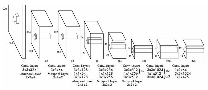
[Figure 5] A YOLO Network Architecture slightly modified by González et al. for galaxy detection
YOLO (You Only Look Once) is a deep learning computer vision algorithm used for object detection in images and videos introduced by Joseph Redmon et al. in 2016. In YOLO, a single neural network predicts bounding boxes and class probabilities directly from full images in one evaluation (single-shot object detection). The basic step-by-step procedure of YOLO network goes as follows.
-
The input image is divided into a grid of cells. The size of the grid is determined by the network architecture and the size of the input image.
-
Each cell is responsible for predicting one or more bounding boxes that contain objects in the image. Each bounding box is represented by a set of 5 values(x, y, w, h, confidence), where the (x, y) coordinates represent the center of the bounding box, (x,h) coordinates represent the width and height of the box, and the confidence value represents the probability that the bounding box contains an object.
-
Each bounding box also has associated class probabilities, which represent the probability that the object within the bounding box belongs to a particular class.
-
The YOLO network uses a single convolutional neural network to simultaneously predict bounding boxes and class probabilities for all cells in the grid. The network is trained on a large dataset of labeled images, using backpropagation to adjust the weights of the network to minimize the prediction error.
-
During inference, the network takes in an input image, processes it through the CNN, and outputs a set of bounding boxes and class probabilities for all cells in the grid, in a single forward pass.
-
After the network outputs the bounding boxes and class probabilities, a post-processing step is applied to filter out low-confidence predictions and non-maximum suppression (NMS) is performed to remove duplicate detections.
-
The remaining bounding boxes are visualized on the input image, along with their associated class probabilities.
4. Training
In YOLO, data augmentation, increasing the training dataset with different transformations of the same data through scaling, rotations, crops, warps, is already implemented. However, in astrophysical context, input images may vary depending on the band-filters and instruments used to obtain the data. Therefore, González et al. trained the YOLO network with 6 different training datasets.
| Name | Dataset | Filters | Images |
|---|---|---|---|
| T1 | S1 | L | 6458 |
| T2 | S1 | LH | 6458 |
| T3 | S2 | L | 11010 |
| T4 | S2 | L+LH+S+SH+Q | 55050 |
| T5 | S2 | LH+SH | 22020 |
| T6 | S2 | L+LH+S+SH+Q | 32290 |
[Table 2] 6 Different Training Datasets used in training AstroCV. Dataset S1 is produced from 7397 field images fetched from the SDSS database and Dataset S2 is produced from 12171 field images, where field images for both S1 and S2 contain at least one galaxy with size larger than 22 pixels (bounding box side). Then different filters have been applied to these two images to increase the size of the training dataset. L stands for Lupton (abovementioned conversion method), LH stands for Lupton High, where the FITS images are converted to RGB images through Lupton method, then the contrast and brightness are enhanced. S and SH stand for sinh and sinh high contrast, and Q stands for sqrt conversion function. Note that sinh and sqrt are quite common conversion functions used in astrophysics (see Figure 6).
[Figure 6-1] Original i-band filter image.

[Figure 6-2] i-band filter image scaled with sinh.
[Figure 6-3] i-band filter image scaled with sqrt.
4-1. Training Results
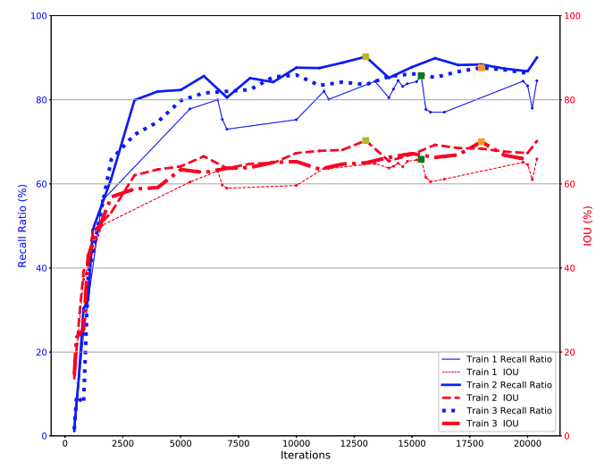
[Figure 7-1] Convergence of T1, T2, and T3 training sets (drawn from González et al.’s paper). The colored squares indicate optimal recall ratio and IOU (Intersection over Union) for the three trainings.
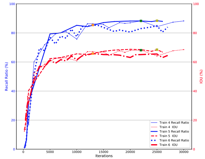
[Figure 7-2] Convergence of T4, T5, and T6 training sets (drawn from González et al’s paper).
González et al stated that the recall and IOU for T4, T5, and T6 (training datasets with more filter augmentations) remain quite similar to the ones for the first three datasets, however, detection and classification is more robust against different conversion functions and instruments.
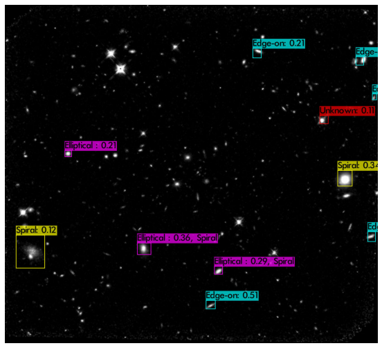
5. YOLO Detections with Pretrained Weights
All of the final results display all the bounding boxes with confidence scores greater than or equal to 0.10.
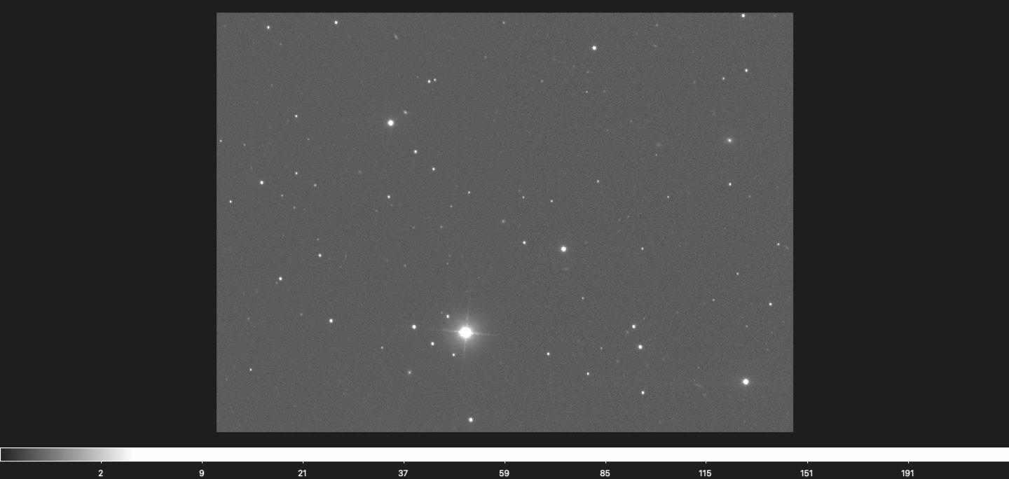
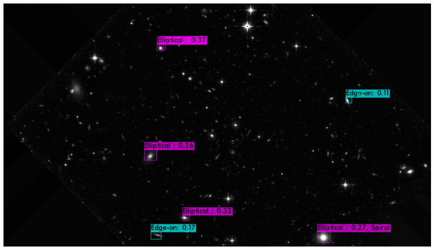
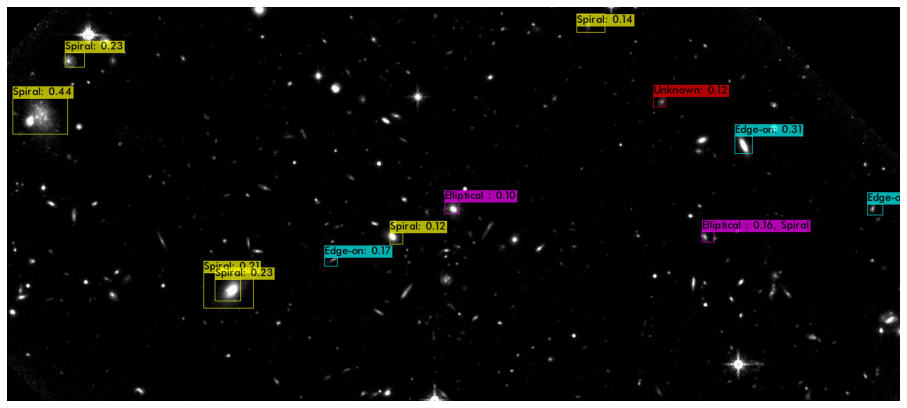
5-1. SDSS Images
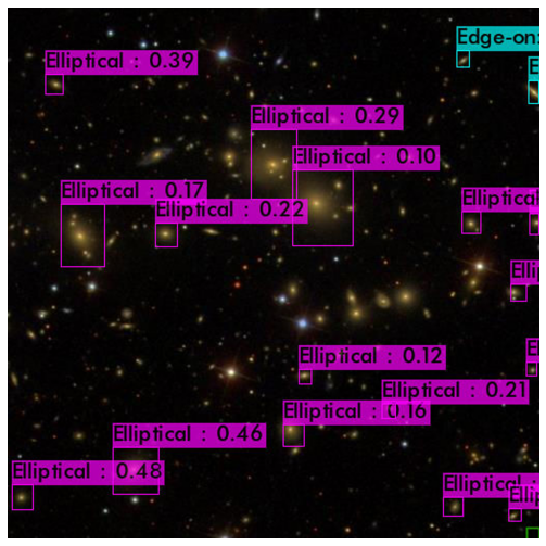
[Figures 8-1, 8-2] Random images drawn from the SDSS database. 8-1 is more zoomed in when compared to 8-2, and resulted in more detected galaxies.
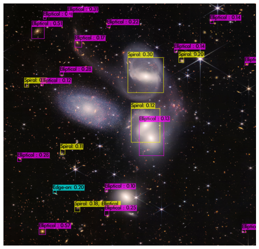
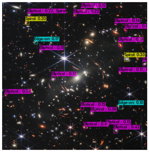
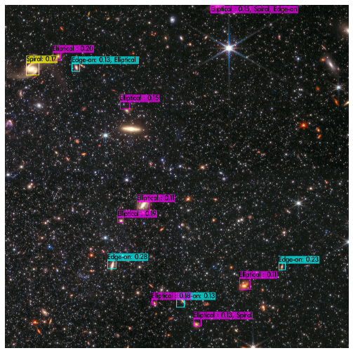
5-2. Hubble Space Telescope Images
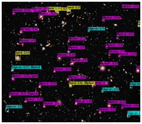
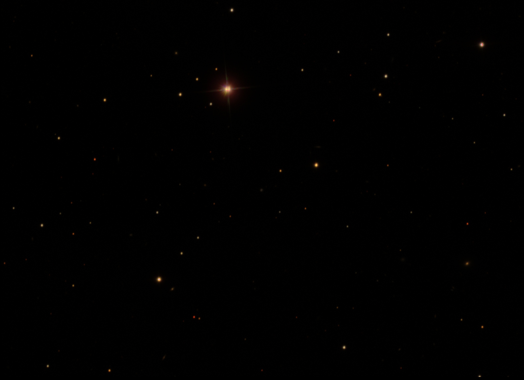
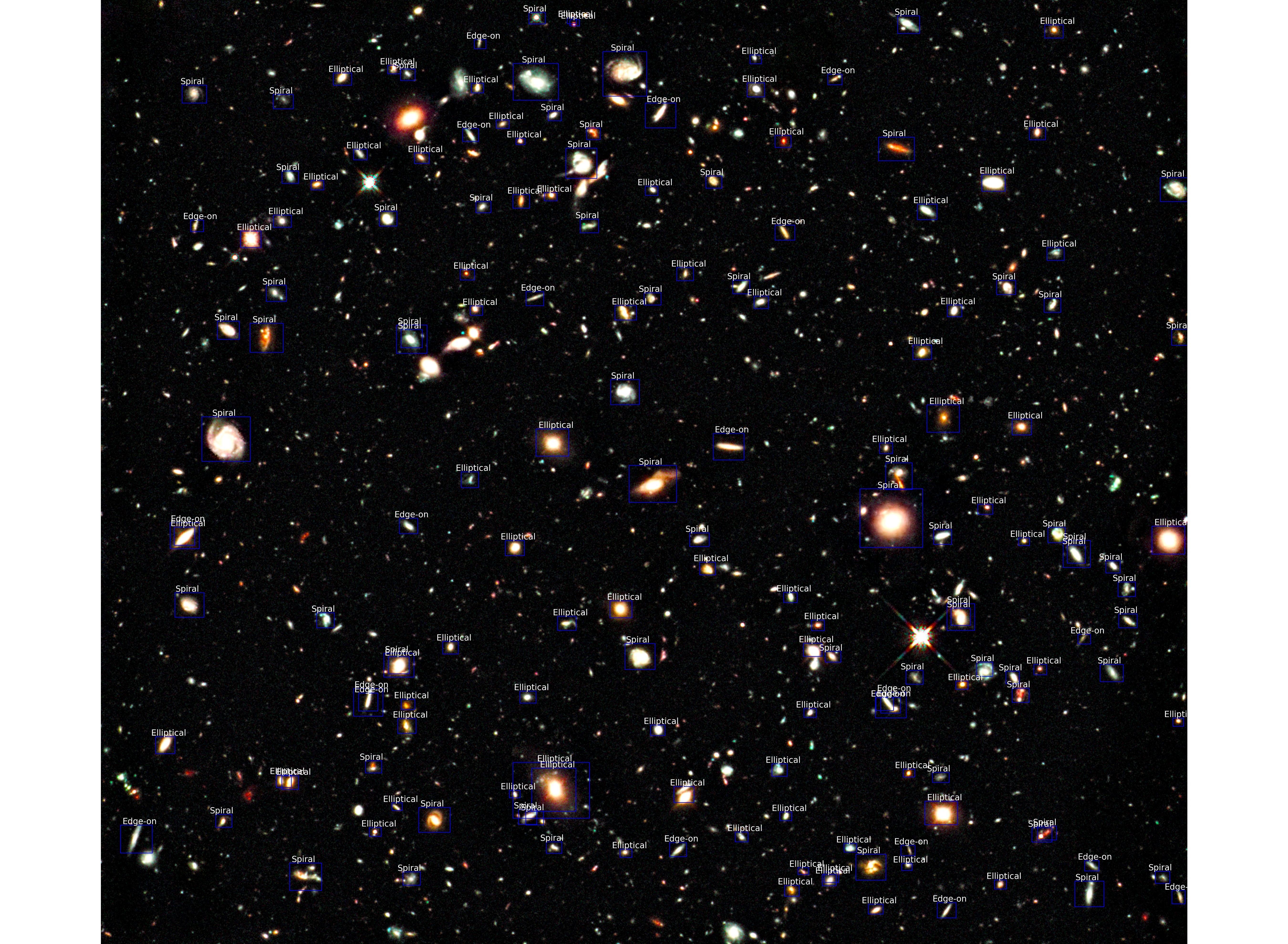
[Figure 9-1] Hubble Deep Field, one of the most famous astronomical picture taken in history. As the image (RGB colored) was generated with postprocessing somewhat similar to Lupton method mentioned above, the model detects/classifies galaxies pretty well.
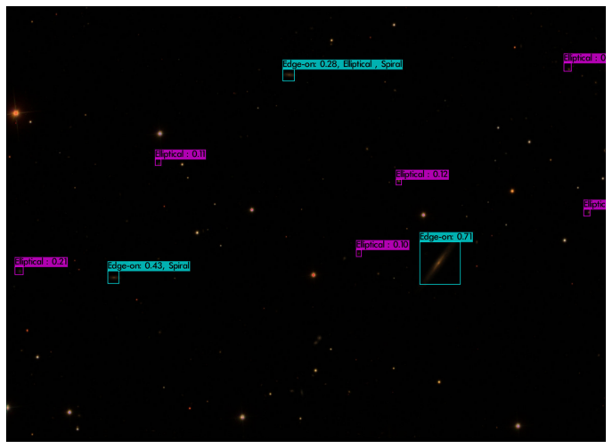
[Figures 9-2, 9-3, 9-4 ] One small section of the universe labeled as R1001ED, taken with the Hubble Space Telescope. This is one of the eight fields that I’m currently working on with Dr. Rich from the Physics and Astronomy department. The three images are from the same field taken with the F160W filter (transmits light in the 1400-1800 nm wavelength range) with different orientations (rotations/scales) and slightly different color scales (SAOImage DS9 supports simple contrast/brightness/color transformations). We can observe that the model performance relies on the instrument, band-filters used to collect data as González et al. stated.
5-3. James Webb Space Telescope Images
[Figure 10-1] Stephan’s Quintet. One of the first images taken with the JWST. It is remarkable that the model detects the two adjacent galaxies in the center but cannot detect the one on the left.
[Figure 10-2] Webb’s First Deep Field, which was unveiled during a White House event on July 11, 2022. Note that the model detects galaxies not around the center, where galaxies are ‘distorted or stretched’ due to the strong gravitational lensing. This addresses a potential research topic in astronomical computer vision; how to deal with images affected by strong gravitation?
[Figure 10-3] One of the most recent JWST images. very fine grained objects. However, due to the limitations of YOLO network, cannot detect small galaxies from the image.
5-4. YOLO-3 based Detection (from AstroCV repo)
[Figure 11] Hubble Deep Field image. Lot more galaxies are detected with a more recent version of YOLO network. This is the last update from the González et al’s github repo, however, there were no pretrained weights available to public.
6. Limitations, Possible Improvements
-
There is no universal conversion method. The conversion method depends on the band filters, and/or the instruments used to collect the data, therefore, the model may not perform very well on the images generated with different conversion methods to the method used in training dataset.
-
Figure 10-2 suggests a very interesting research topic; how to deal with the gravitational lensing? Can we train the model to detect (not visually, but detect the presence of) very massive objects (i.e. black hole) from the image through severe distortions in galaxies? After the model is trained to detect massive objects, can we train the model to detect galaxies with uncommon shapes?
-
YOLO is known for its advantages in real-time detections. The main purpose of González et al’s paper was to investigate any possibilities to use YOLO algorithm to detect astronomical objects in real-time observations. However, if we are trying to detect astronomical objects in non-synchronous environment (from images already taken), can two-stage detection algorithms (e.g. R-CNN) outperform YOLO based detection algorithm in astrophysical context?
- There is one paper tried to use R-CNN to detect low surface brightness galaxies (https://par.nsf.gov/servlets/purl/10340970)
- There is one paper tried to use R-CNN to detect low surface brightness galaxies (https://par.nsf.gov/servlets/purl/10340970)
7. Discussion
Even though space science research generates TBs of data every day, due to its complexity, attempts to integrate deep-learning computer vision models have been extremely rare. The paper that I heavily relied on, González et al’s Galaxy Detection and Identification Using Deep Learning and Data Augmentation, is one of the very first papers that tried to integrate modern computer vision algorithms into astrophysical research. However, after the launch of JWST last year and the expected launch of Rubin Observatory (previously named, LSST) in 2024, there’s a growing expectation and interest in integrating computer vision deep learning algorithms into astrophysics. (List of more modern papers in astro-computer vision: https://github.com/georgestein/ml-in-cosmology#structure). As a student who majored in both computer science and astrophysics, willing to pursue an academic career in astrophysics, I wish I could use novel computer vision algorithms into my research later in the future.
You can find the link code I used at AstroCV, and gdrive
Relevant Papers
[1] Star-Galaxy Classification Using Deep Convolutional Neural Networks
- https://ui.adsabs.harvard.edu/abs/2017MNRAS.464.4463K/abstract
- https://github.com/EdwardJKim/dl4astro
Conventional star-galaxy classifiers use the reduced summary information from catalogues with carefully selected features (by human). The paper introduces the possibility of using deep convolutional neural networks (ConvNets) to automatically learn the features directly from the data which minimizes the input from human researchers.
[2] Machine Learning Classification of SDSS Transient Survey Images
- https://ui.adsabs.harvard.edu/abs/2015MNRAS.454.2026D/abstract
The paper tests performance of multiple machine learning algorithms in classifying transient imaging data from the Sloan Digital Sky Survey (SDSS) into real objects and artefacts.
[3] Galaxy Detection and Identification Using Deep Learning and Data Augmentation
- https://ui.adsabs.harvard.edu/abs/2018A%26C….25..103G/abstract
- https://github.com/astroCV/astroCV
The paper introduces a novel method for automatic detection and classificaiton of galaxies to make trained models more robust against the data taken from different instruments as part of AstroCV.
References
[1] Kim, E. J. and Brunner, R. J., “Star-galaxy classification using deep convolutional neural networks”, Monthly Notices of the Royal Astronomical Society, vol. 464, no. 4, pp. 4463–4475, 2017. doi:10.1093/mnras/stw2672.
[2] du Buisson, L., Sivanandam, N., Bassett, B. A., and Smith, M., “Machine learning classification of SDSS transient survey images”, Monthly Notices of the Royal Astronomical Society, vol. 454, no. 2, pp. 2026–2038, 2015. doi:10.1093/mnras/stv2041.
[3] González, R. E., Muñoz, R. P., and Hernández, C. A., “Galaxy detection and identification using deep learning and data augmentation”, Astronomy and Computing, vol. 25, pp. 103–109, 2018. doi:10.1016/j.ascom.2018.09.004.
[4] Lupton, R., Blanton, M. R., Fekete, G., Hogg, D. W., O’Mullane, W., Szalay, A., & Wherry, N. (2004). Preparing Red‐Green‐Blue Images from CCD Data. Publications of the Astronomical Society of the Pacific, 116(816), 133–137.
[5] J. Redmon, S. Divvala, R. Girshick and A. Farhadi, “You Only Look Once: Unified, Real-Time Object Detection,” in 2016 IEEE Conference on Computer Vision and Pattern Recognition (CVPR), Las Vegas, NV, USA, 2016 pp. 779-788.
doi: 10.1109/CVPR.2016.91