U-Net for Biomedical Image Segmentation
This report dives into the aspect of biomedical image segmentation, using U-Net and U-Net 3D. U-Net revolutionized the field with its unique U-shaped architecture designed for precise semantic segmentation, while 3D U-Net tackled 3D images, enhancing efficiency and accuracy in 3D segmentation compared the regular U-Net.
- Introduction
- Before Deep Learning
- Model #1: U-Net for 2D image segmentation
- Model #2: U-Net 3D for 3D Image Segmentation
- Discussion
- Conclusion
- Reference
Introduction
Medical image segmentation enable the detailed analysis of images obtained from various modalities such as microscopy, MRI, and CT scans. The advancement of medical image segmentation not only helped with medical fields, but also advance computer vision segmentation technology in general. Traditionally, medical image segmentation relied on manual annotation, the process was not only labor-intensive but also prone to inconsistency. The emergence of deep learning technologies, particularly the U-Net architecture introduced in 2015 by Olaf Ronneberger, Philipp Fischer, and Thomas Brox, marked a significant advancement in this field. U-Net, with its unique structure, efficiently addresses both the need for detailed segmentation of biomedical images and the challenges posed by limited data availability. It employs a symmetric architecture with skip connections to enhance the flow of information, allowing for precise segmentation results. Following its success, 3D U-Net was developed to extend its application to volumetric data, further solidifying its utility in medical image analysis. This report aims to explore the development, architecture, and impact of U-Net and its variants in the realm of biomedical image segmentation.
Before Deep Learning
Before deep learning became widely used, several traditional methods were used for medical picture segmentation. These methods were mostly based on mathematical models and image processing.
- Thresholding Techniques in Image Segmentation
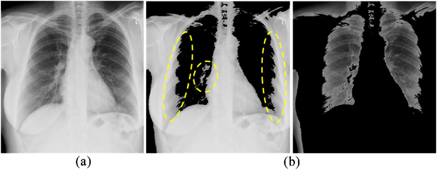 Image from Matsuyama’s “A Novel Method for Automated Lung Region Segmentation in Chest X-Ray Images” [9]
One of the fundamental methods of picture segmentation is thresholding. This technique divides pixels into foreground and background based on their intensity levels, which streamlines the segmentation process. It works especially well in situations where you need to identify lesions in medical photos or differentiate between different tissues. Finding the ideal threshold value is the main obstacle in thresholding, though, particularly in complicated images where the difference between several regions can be slight.
- Region Growing for Connected Structure Segmentation
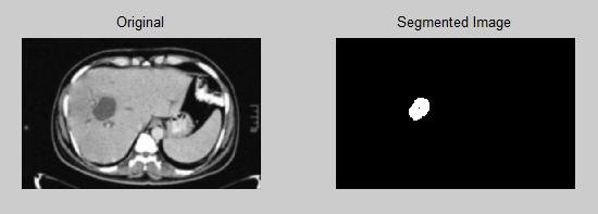 Image from “Automatic Detection of Abnormalities Associated with Abdomen and Liver Images” [10]
Another important strategy is called Region Growing; it starts with one or more seed points and grows by adding nearby pixels that satisfy certain requirements, including intensity similarity. This method works well for segmenting areas of similar intensity or related structures within a picture. However, the segmentation accuracy is affected by noise, and choosing the right seed locations continues to be a significant difficulty.
- Clustering Algorithms in Medical Image Analysis
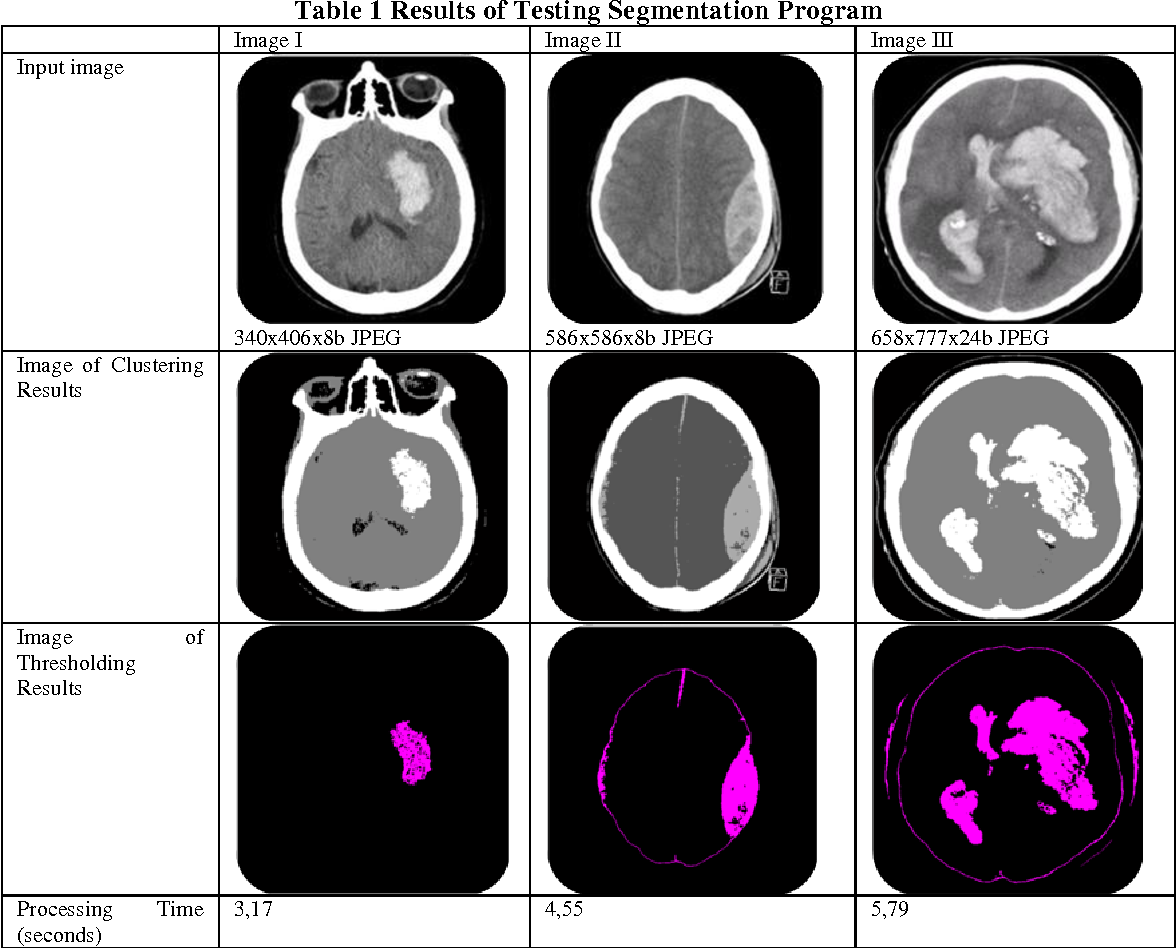 Image from “Nurhasanah et al. “Image Segmentation Of CT Head Image To Define Tumour Using K-Means Clustering Algorithm.” [11]
Medical picture segmentation also relies heavily on clustering methods like KMeans, which allow pixels to be grouped into clusters based on feature similarities without the need for starting seeds. By repeatedly adjusting pixels to the nearest cluster center, this technique maximizes the homogeneity of the clusters. It has shown to be very useful for classifying tissues and identifying anomalous areas in medical imaging. Notwithstanding its effectiveness, the main obstacles are figuring out the ideal number of clusters and handling different cluster sizes, which might affect the quality of segmentation.
- Watershed Algorithm for Separating Adjacent Objects
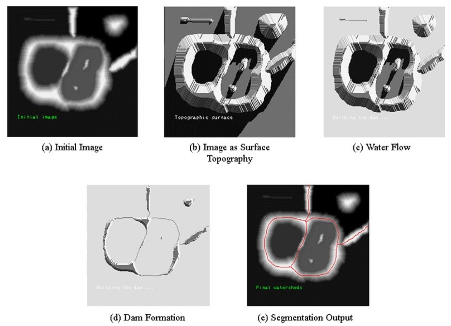 Image from “Amoda, Niket & Kulkarni, Ramesh. (2013)’s Efficient Image Segmentation Using Watershed Transform” [12]
The gradient in the image is treated as a topographic surface using the Watershed Algorithm, which uses a novel approach. Watershed lines, which distinguish several catchment basins, provide the basis for the picture segmentation. This feature is very helpful in distinguishing touching things, like cells in microscopic images. The watershed method, although novel in its approach, is vulnerable to over-segmentation, which is frequently intensified by noise and local imperfections within the image.
- Edge Detection for Detailed Structure Outlining
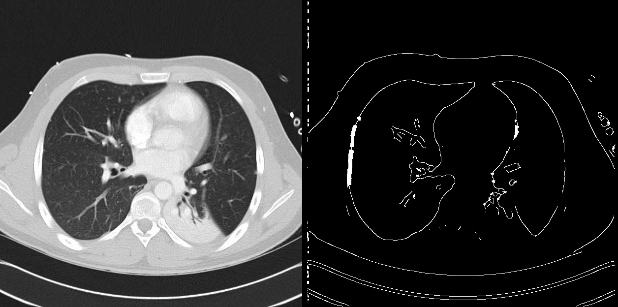 Image from Krzisnik’s “Edge Detection Archives” [13]
By detecting boundaries through intensity discontinuities, edge detection algorithms are essential to the segmentation of medical images. This method helps with thorough anatomical and pathological examinations by precisely delineating organs, tumors, or other anatomical features. However, there are issues with edge recognition techniques, such as their susceptibility to picture noise, which can cause them to overlook tiny edges or identify ones that are fake. The algorithm’s capacity to discern between real edges and noise is a major factor in edge detection efficacy.
- Active Contours for Precise Boundary Detection
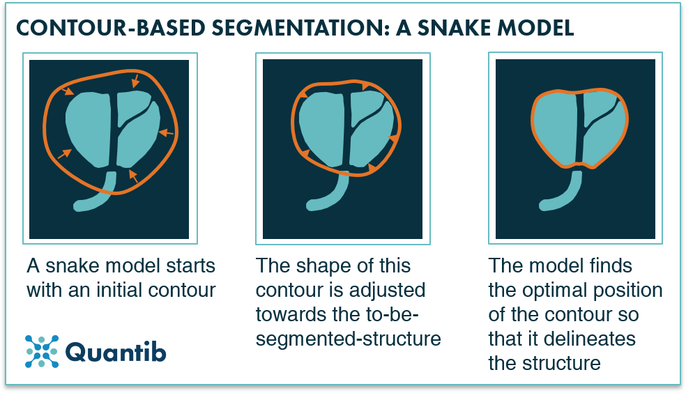 Image from Moeskops’s “Deep Learning Applications in Radiology: Image Segmentation.” [14]
Active Contours, sometimes known as Snakes, are a dynamic way to identify object boundaries in a picture. These contours are computer models that develop over time to precisely define object contours, particularly in intricate settings. For accurately delineating organs, tumors, or other structures, active contours are useful. They do, however, present serious issues in terms of computational resources and user intervention because they are computationally demanding and require manual initialization.
The improvements in medical imaging can be largely attributed to the use of classical methods for medical picture segmentation. Nevertheless, they pose particular difficulties that restrict their effectiveness, especially when processing intricate medical images. These difficulties include the need for human tuning and initialization, sensitivity to noise and fluctuation, and limited ability to handle complex structures.
-
Sensitivity to Noise and Variability Certain techniques are more susceptible to noise and unpredictability in picture data than others, including the Watershed Algorithm and Edge Detection. Because of their sensitivity, they may not be able to accurately segment complicated medical images when accuracy is crucial. For example, in images with small contrast differences, edge detection might not be able to distinguish boundaries effectively, and in noisy images, the watershed approach might cause over-segmentation.
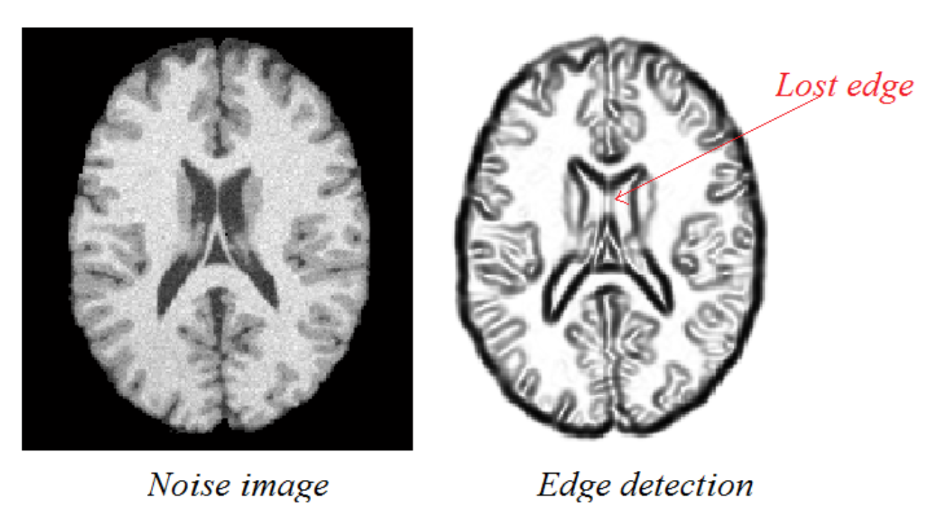 Image from “Best Method to Find Edge of Noise Image.” [15]
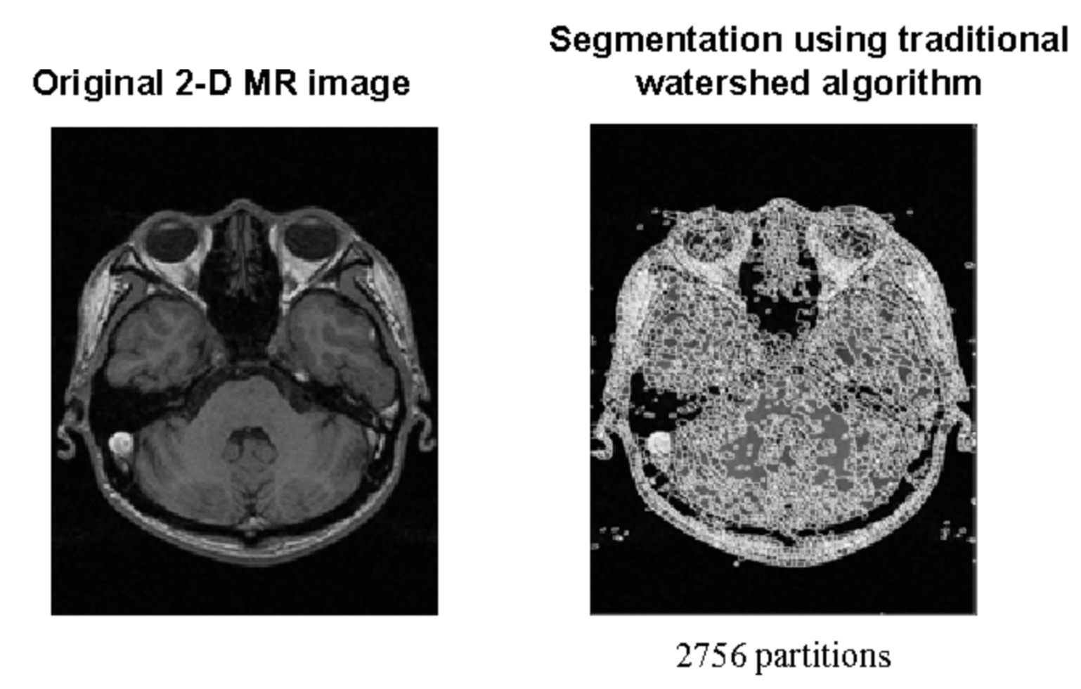 Image from “Medical Image Segmentation Using K-Means Clustering and Improved Watershed Algorithm.” [16]
 - Need for Manual Tuning and Initialization Approaches such as Region Growing and Active Contours require a large amount of human labor to initialize and adjust settings. This requirement not only increases the labor intensity involved in the segmentation process, but it also reduces the automation of these procedures. Both active contours and region growth need the placement of a beginning curve in close proximity to the object of interest and the appropriate selection of seed points, respectively. These are crucial phases that impact the final segmentation result. Restricted Ability to Manage Complicated Structures
- Limited Capability in Handling Complex Structures Complex biological structures frequently pose challenges for classical segmentation approaches, requiring either sophisticated adaptations to the basic algorithms or substantial preprocessing. The segmentation task may get more complex due to diseases and the inherent heterogeneity of anatomical components among individuals. Because of this, it is frequently necessary to customize and manually intervene in order to achieve correct segmentation of complicated structures, which can be difficult in clinical contexts.
These difficulties highlight the shortcomings of traditional segmentation techniques and the demand for more reliable, automated techniques that can handle the intricacies of medical imaging. These issues have started to be addressed by the development of deep learning and convolutional neural networks, which has revolutionized medical image segmentation, offering significant improvements over classical approaches:
- Automatic Feature Learning: Without the requirement for human feature selection, deep learning algorithms are excellent at extracting pertinent features from data directly.
- Robustness to Noise: By nature, these models are more resilient to image artifacts and noise, which improves segmentation accuracy.
- Managing complicated Structures: Deep learning models are able to handle complicated anatomical structures with greater ease than traditional methods because they have the capacity to build hierarchical representations.
- Enhanced Accuracy and Efficiency: U-Net and similar technologies interpret images more quickly and accurately, minimizing the need for human intervention.
Model #1: U-Net for 2D image segmentation
U-Net is a special type of architecture that makes use of convolutional layers and max pooling. It is designed for image semantic segmentation purpose and is very effective in segmenting biomedical images. U-Net was proposed in 2015 in the paper “U-Net: Convolutional Networks for Biomedical Image Segmentation” by Olaf Ronneberger, Philipp Fischer, and Thomas Brox. Using this architecture, they won the Cell Tracking Challenges as of ISBI 2015.
Dataset
The U-Net paper utilized datasets from both the IEEE International Symposium on Biomedical Imaging (ISBI) 2012 and ISBI 2015 challenges.
In this report, I also use the database from CVC Clinic DB for colon polyps and run the code based on this database to segment the polyps from the images.
ISBI Challenge 2012 - EM stacks
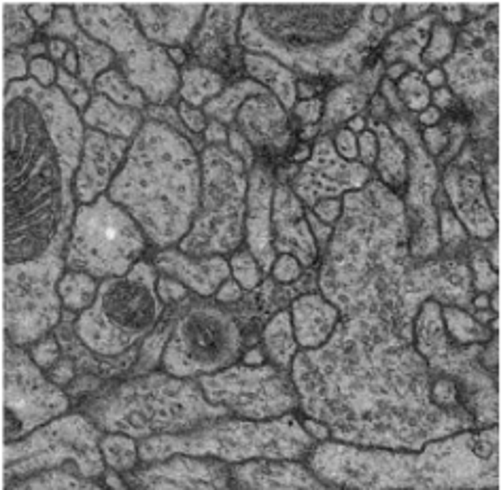
During the ISBI 2012, a challenge workshop focusing on the segmentation of neuronal structures within electron microscopy (EM) stacks was conducted. This challenge provided participants with a complete set of EM slices to develop and train machine-learning models for the automated segmentation of neural structures. [1]
ISBI Challenge 2015 - Cell tracking
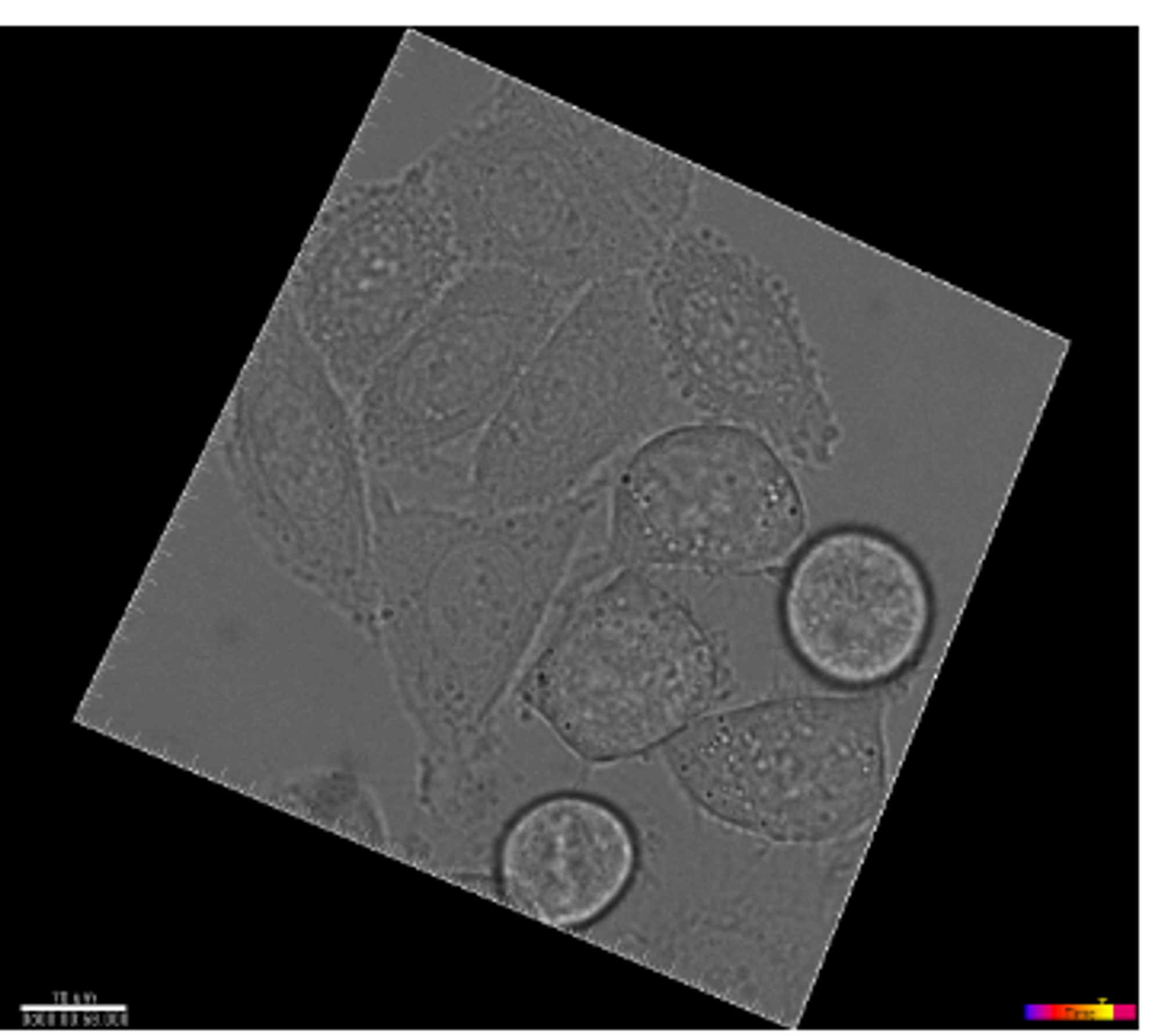
For the ISBI cell tracking challenge for the years 2014 and 2015. The challenge’s dataset features time-lapse imagery that captures the dynamics of cell or nucleus movement in both two and three dimensions, on surfaces or within substrates. Additionally, it includes 2D and 3D video data of synthetically generated fluorescent cells and nuclei, showcasing a variety of shapes and movement patterns, available at http://celltrackingchallenge.net/datasets/. [2]
CVC Clinic DB (For colon polyps)
CVC-ClinicDB is an open-access dataset of 612 images with a resolution of 384×288 from 31 colonoscopy sequences. It is used for medical image segmentation, particularly polyp detection in colonoscopy videos. [3]
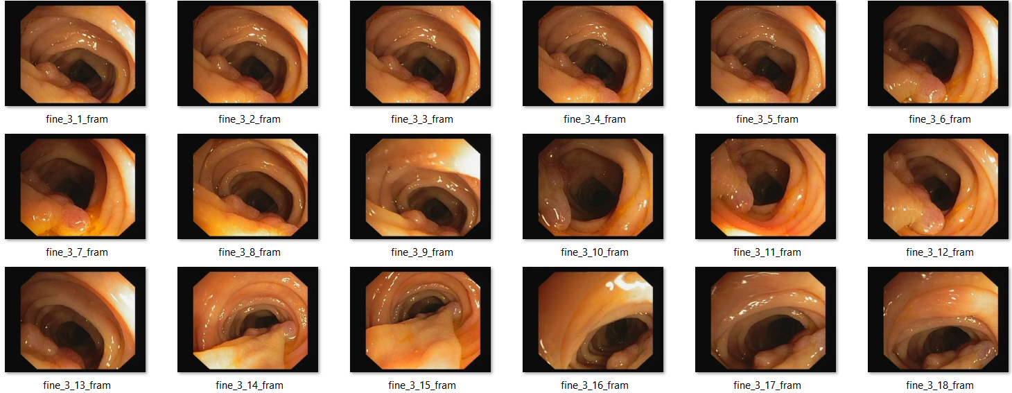
Processing data: Data augmentation
Data augmentation plays a crucial role in imparting desired invariance and robustness properties to the network, especially when the training dataset is limited. To achieve this, we create smooth deformations by applying random displacement vectors across a coarse 3 by 3 grid. [4]
For example: These are the same images after some modification.

Code implementation for data augmentation :
In this code [5], ImageDataGenerator(**aug_dict) is responsible for applying data augmentation techniques to both the input images and their corresponding masks.
image_datagen = ImageDataGenerator(**aug_dict)
image_generator = image_datagen.flow_from_directory(
        train_path,
        classes = [image_folder],
        class_mode = None,
        color_mode = image_color_mode,
        target_size = target_size,
        batch_size = batch_size,
        save_to_dir = save_to_dir,
        save_prefix  = image_save_prefix,
        seed = seed)
Architecture
This is the demonstration of U-Net architecture [4]

UNet consists of:
- A Contracting path (Downsampling/Encoder) (left): Consists of two 3x3 covolutions, each followed by a ReLU and a 2x2 max pooling operation with stride 2 for downsampling. When downsampling, we also double the number of feature channels. We keep repeating this
- Skip connection that connect the 2 paths to retain fine detail due to the loss of border pixels in every convolution. We get the result of the last layer of each step in the left side and add it to the corresponding one in the right side.
- An Expansive path (Upsampling/ Decoder) (right): At each step in expansive path, we upsample the feature map followed by a 2x2 convolution that halves the number of feature channels, and two 3x3 convolutions, each followed by a ReLU. Then we keep repeating this. At the end, we use a 1x1 convolution to map each 64 component feature to the desired number of classes. [4]
Code implementation for UNet
This code [6] defines a convolutional block (conv_block) and a function (build_unet_model) to construct a U-Net model for image segmentation. The conv_block function applies two convolutional layers with batch normalization and ReLU activation. The build_unet_model function constructs the U-Net architecture, consisting of an encoder, bridge, and decoder stages with skip connections, followed by a convolutional layer with sigmoid activation for segmentation output.
def conv_block(x, num_filters):
    x = Conv2D(num_filters, (3, 3), padding="same")(x)
    x = BatchNormalization()(x)
    x = Activation("relu")(x)

    x = Conv2D(num_filters, (3, 3), padding="same")(x)
    x = BatchNormalization()(x)
    x = Activation("relu")(x)

    return x

def build_unet_model():
    size = 256
    num_filters = [16, 32, 48, 64]
    inputs = Input((size, size, 3))

    skip_x = []
    x = inputs
    ## Encoder
    for f in num_filters:
        x = conv_block(x, f)
        skip_x.append(x)
        x = MaxPool2D((2, 2))(x)

    ## Bridge
    x = conv_block(x, num_filters[-1])

    num_filters.reverse()
    skip_x.reverse()
    ## Decoder
    for i, f in enumerate(num_filters):
        x = UpSampling2D((2, 2))(x)
        xs = skip_x[i]
        x = Concatenate()([x, xs])
        x = conv_block(x, f)

    ## Output
    x = Conv2D(1, (1, 1), padding="same")(x)
    x = Activation("sigmoid")(x)

    return Model(inputs, x)
To build the model, run:
model = build_unet_model()
model.evaluate(test_dataset, steps=test_steps)
Training details and Loss Function
Unet is optimized using Stochastic Gradient Descent with Momentum \(\textit{n} = 0.99\). The original Unet was trained with batch size = 1 due to the small size of GPU’s RAM at the time.
\[\textit{v}_t = \textit{y}\textit{v}_{t-1} + \textit{n}\nabla\textit{w}_t\] \[\textit{w}_{t+1} = \textit{w}_t - \textit{v}_t\]During training, Unet attempt to optimize the energy function
\[E = \sum_{x\in\Omega}^{}\textit{w}(x)log(p_{l(x)}(x))\]\(l(x)\) returns the ground-truth label for the pixel x. So we can see the objective function is punishing wrong pixel classification. However, not every wrong pixel is punished equally.
\(\textit{w}(x)\) is a pre-computed weight map for each segmentation map. Notice that \(\textit{w}(x)\) is pre-computed and not trainable. Using the pre-computed weight map, we will punish more heavily wrong classification for pixels at the border region. Below is a picture for the pre-computed weight map, you can see the border pixels are highlighted. [4]
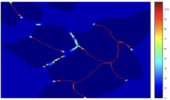 (This image is from Ronneberger Olaf’s paper [4])
Results
UNet results in the challenges
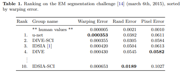
In 2015, the UNet architecture demonstrated remarkable success in two challenges: the EM (Electron Microscopy) Segmentation Challenge and the ISBI Cell Tracking Challenge. UNet’s performance in these challenges solidified its reputation as a powerful tool for semantic segmentation tasks in biomedical image processing. [4]

Code implementation results
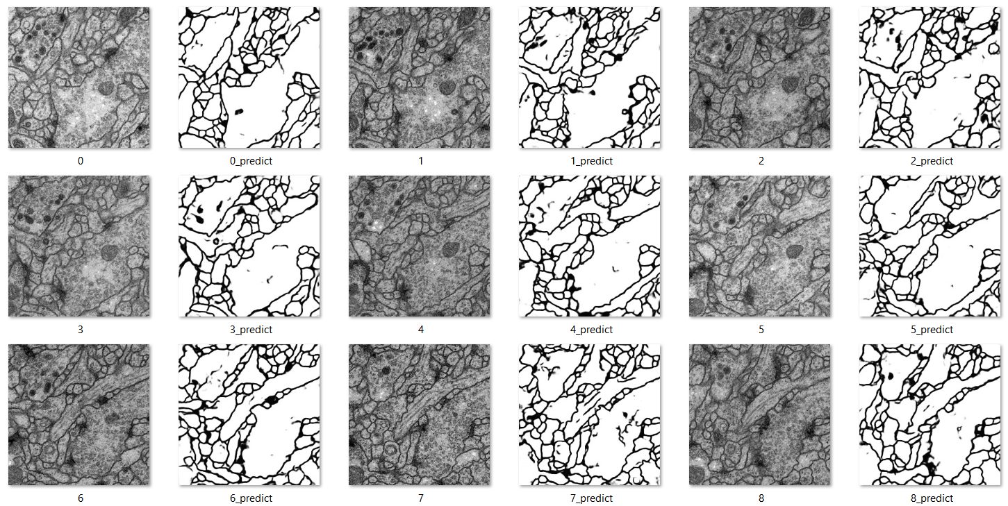
For ISBI 2012: Training: This code [5] sets up data augmentation parameters such as rotation, shifting, shearing, zooming, and flipping for training images. It then generates training data using a custom generator trainGenerator, initializes a U-Net model, and trains it for 5 epochs with 2000 steps per epoch, saving the best model using ModelCheckpoint.
data_gen_args = dict(rotation_range=0.2,
                    width_shift_range=0.05,
                    height_shift_range=0.05,
                    shear_range=0.05,
                    zoom_range=0.05,
                    horizontal_flip=True,
                    fill_mode='nearest')
myGene = trainGenerator(2,'data/membrane/train','image','label',data_gen_args,save_to_dir = None)
model = unet()
model_checkpoint = ModelCheckpoint('unet_membrane.hdf5', monitor='loss',verbose=1, save_best_only=True)
model.fit_generator(myGene,steps_per_epoch=2000,epochs=5,callbacks=[model_checkpoint])
Then run the trained model, we get these predictions that are saved into a file:
For CVC-612 (Colon Polyps)
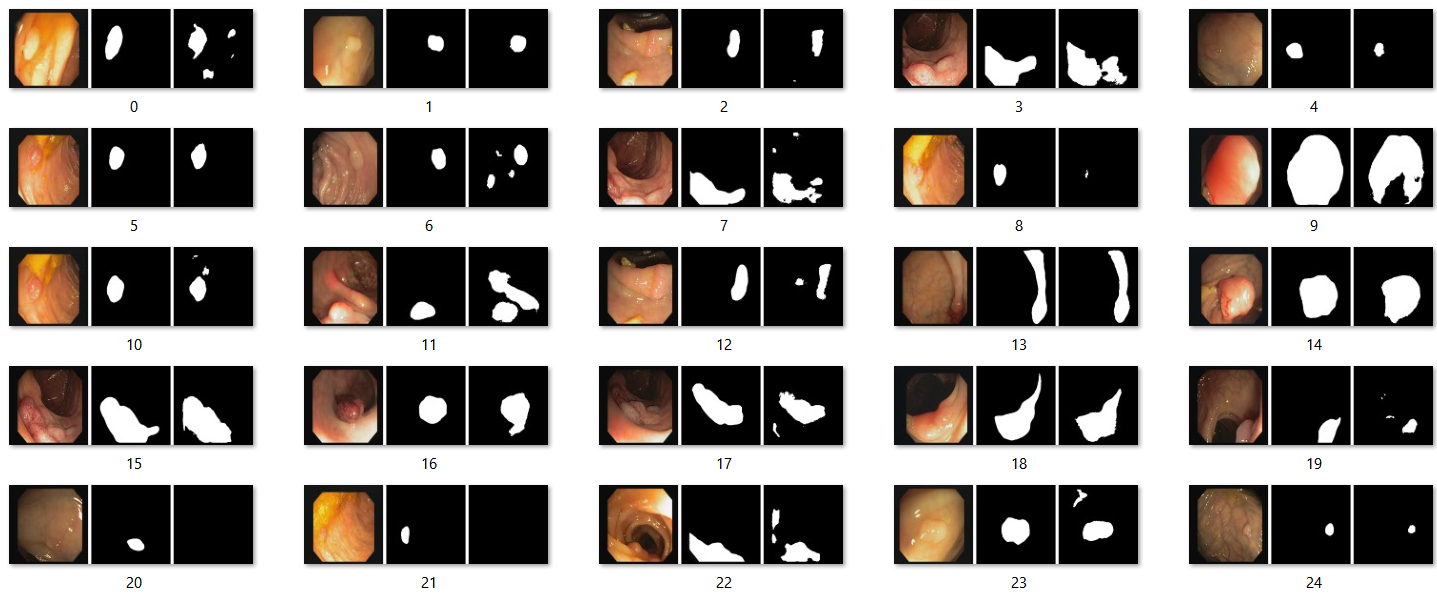
Code implementation to train the model [6]. Here we also use Adam with learning rate of 1e^-4
## Hyperparameters
    batch = 8
    lr = 1e-4
    epochs = 20

    train_dataset = tf_dataset(train_x, train_y, batch=batch)
    valid_dataset = tf_dataset(valid_x, valid_y, batch=batch)

    model = build_model()

    opt = tf.keras.optimizers.Adam(lr)
    metrics = ["acc", tf.keras.metrics.Recall(), tf.keras.metrics.Precision(), iou]
    model.compile(loss="binary_crossentropy", optimizer=opt, metrics=metrics)

    callbacks = [
        ModelCheckpoint("files/model.h5"), ReduceLROnPlateau(monitor='val_loss', factor=0.1, patience=4), CSVLogger("files/data.csv"), TensorBoard(), EarlyStopping(monitor='val_loss', patience=10, restore_best_weights=False)
    ]
    train_steps, valid_steps = len(train_x)//batch, len(valid_x)//batch
    if len(train_x) % batch != 0: train_steps += 1
    if len(valid_x) % batch != 0: valid_steps += 1

    model.fit(train_dataset, validation_data=valid_dataset, epochs=epochs, steps_per_epoch=train_steps, validation_steps=valid_steps, callbacks=callbacks)
Run the model, the results are saved in to a file. The first image is the original image, the second one is the ground truth and the third image is the prediction.
Model #2: U-Net 3D for 3D Image Segmentation
Followed by the success of 2D U-Net, 3D U-Net was proposed in the following paper: “3D U-Net: Learning Dense Volumetric Segmentation from Sparse Annotation”. We can still use 2D U-Net on 3D images by analyzing each slices of the images. However, this is very inefficient. Therefore, 3D U-Net suggests a deep network that can generate dense volumetric segmentation that only requires some annotated 2D for training.
Architecture
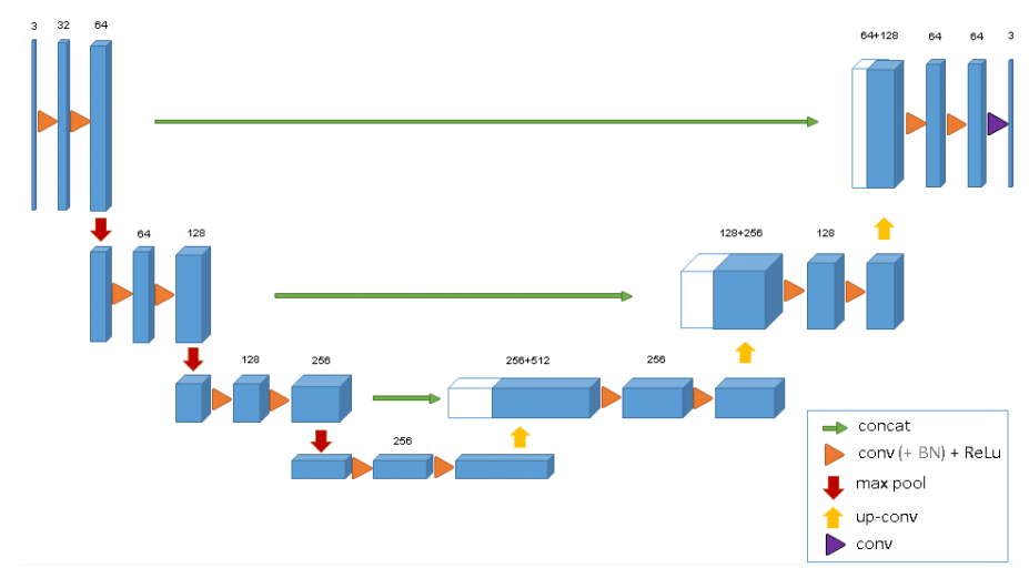 3D U-Net architecutre: Blue boxes are feature maps with number of channels above them. [7]
Similar to the regular U-Net, it has the U structure, two paths: downsampling, upsampling, and skip connections.
The difference will be the dimension. For each downsampling step, each layer contains two 3x3x3 convolutions, each followed by a ReLU, and then a 2x2x2 max pooling with stride = 2. For upsampling process, each layer consists of an upconvolution of 2x2x2 with stride = 2, followed by two 3x3x3 convolutions, each followed by a ReLU. The skip connetions from layers of equal resolution provides the essential high-resolution features o the expansive path. [7]
Another difference is also doubling the number of channels before max pooling to avoid bottlenecks. We also introduce batch normalization before each ReLU. [7]
Code implementation for U-Net 3D Model [8]:
def conv_block(input, num_filters):
    x = Conv3D(num_filters, 3, padding="same")(input)
    x = BatchNormalization()(x)   #Not in the original network.
    x = Activation("relu")(x)

    x = Conv3D(num_filters, 3, padding="same")(x)
    x = BatchNormalization()(x)  #Not in the original network
    x = Activation("relu")(x)

    return x

#Encoder block: Conv block followed by maxpooling


def encoder_block(input, num_filters):
    x = conv_block(input, num_filters)
    p = MaxPooling3D((2, 2, 2))(x)
    return x, p

#Decoder block
#skip features gets input from encoder for concatenation

def decoder_block(input, skip_features, num_filters):
    x = Conv3DTranspose(num_filters, (2, 2, 2), strides=2, padding="same")(input)
    x = Concatenate()([x, skip_features])
    x = conv_block(x, num_filters)
    return x

#Build Unet using the blocks
def build_unet(input_shape, n_classes):
    inputs = Input(input_shape)

    s1, p1 = encoder_block(inputs, 64)
    s2, p2 = encoder_block(p1, 128)
    s3, p3 = encoder_block(p2, 256)
    s4, p4 = encoder_block(p3, 512)

    b1 = conv_block(p4, 1024) #Bridge

    d1 = decoder_block(b1, s4, 512)
    d2 = decoder_block(d1, s3, 256)
    d3 = decoder_block(d2, s2, 128)
    d4 = decoder_block(d3, s1, 64)

    if n_classes == 1:  #Binary
      activation = 'sigmoid'
    else:
      activation = 'softmax'

    outputs = Conv3D(n_classes, 1, padding="same", activation=activation)(d4)  #Change the activation based on n_classes
    print(activation)

    model = Model(inputs, outputs, name="U-Net")
    return model
Build the model [8]:
model = build_unet((patch_size,patch_size,patch_size,channels), n_classes=n_classes)
#For example: my_model = build_unet((64,64,64,3), n_classes=4)
Training
Rotation, scaling, and gray value segmentation techniques are applied to both the data and ground truth labels. A smooth dense deformation is then applied to ensure alignment.
The network output and ground truth labels are evaluated using softmax with weighted cross-entropy loss. This involves adjusting the weights to reduce the influence of frequently occurring background voxels and increase the influence of inner tubule voxels, achieving a balanced impact on the loss function. Additionally, setting the weights of unlabeled pixels to zero enables the model to learn solely from labeled data, facilitating generalization across the entire volume. This is how it can helps increase the efficiency when working with 3D images. [7]
Data:
For the code implementation, we have a dataset of sandstones, with dimension of 256 x 256 x 256, which means, there are 256 slices of images size 256 x 256.
We then process the data by break it into patches of 64x64x64 for training.
The dataset can be downloaded here: https://github.com/bnsreenu/python_for_image_processing_APEER
Results
We do training [8] on the given 64 slices of the 3D images and save that train model
#Fit the model
history=model.fit(X_train,
          y_train,
          batch_size=8,
          epochs=100,
          verbose=1,
          validation_data=(X_test, y_test))
Use that model to run the code on those 64 slices, we can get something like this for each slide:
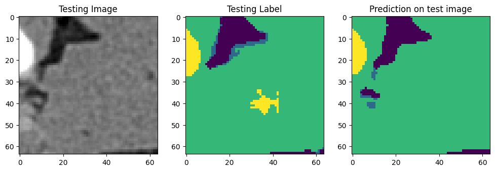
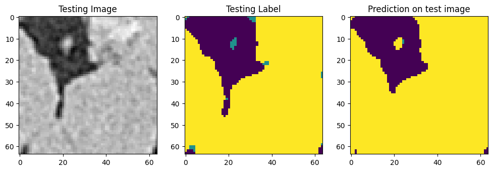
We can now segment the full volume using the trained model. [8]
#Break the large image (volume) into patches of same size as the training images (patches)
large_image = io.imread('/content/drive/MyDrive/Colab Notebooks/sandstone_data_for_ML/data_for_3D_Unet/448_images_512x512.tif')
patches = patchify(large_image, (64, 64, 64), step=64)  #Step=256 for 256 patches means no overlap
print(large_image.shape)
print(patches.shape)

# Predict each 3D patch
predicted_patches = []
for i in range(patches.shape[0]):
  for j in range(patches.shape[1]):
    for k in range(patches.shape[2]):
      #print(i,j,k)
      single_patch = patches[i,j,k, :,:,:]
      single_patch_3ch = np.stack((single_patch,)*3, axis=-1)
      single_patch_3ch = single_patch_3ch/255.
      single_patch_3ch_input = np.expand_dims(single_patch_3ch, axis=0)
      single_patch_prediction = my_model.predict(single_patch_3ch_input)
      single_patch_prediction_argmax = np.argmax(single_patch_prediction, axis=4)[0,:,:,:]
      predicted_patches.append(single_patch_prediction_argmax)
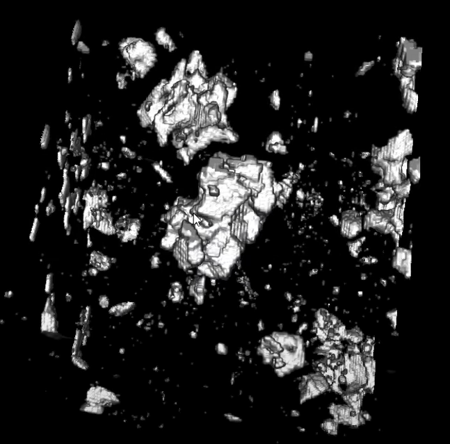
From this implementaion, we get the dimension of the results as: (448, 64, 64, 64)
Which means, from 64 slices, we get 448 after predicting the 3d patch.
Results:
Discussion
U-Net, introduced in 2015, revolutionized medical image segmentation with its efficient architecture. Its 3D variant, proposed in 2016, further extended its capabilities. Despite their age, both versions remain highly effective for addressing medical image segmentation challenges.
While U-Net excels with 2D images, its efficiency diminishes when applied to 3D due to the need to slice volumetric data. This process significantly increases computational demands and complexity.
The introduction of U-Net 3D addresses this issue by efficiently handling volumetric data, even with limited training samples. Its ability to generate more data from a smaller data set mitigates the challenge of sparse medical image repositories.
Talking about how U-Net 3D can generate the lacking data from the existing data, we also think of the difficulty of collecting medical images and the ground truth labels, especially when it comes to 3D images. It is a tedious process to manually go through all hundreds of slices to get the ground truth of the data. We can use data augmentation to generate more data, of course, but we can make use of some unsupervised learning techniques:
- Generative Adversarial Networks (GANs): By training a GAN on a dataset of real medical images, the generator network learns to produce realistic synthetic images, while the discriminator network learns to differentiate between real and synthetic images. Through this adversarial process, GANs can generate high-fidelity medical images that closely resemble real data.
- Variational Autoencoders (VAEs): VAEs learn a latent space representation of the input data, enabling the generation of new samples by sampling from this learned distribution. By training VAEs on large datasets of medical images, researchers can generate diverse and realistic synthetic images that capture the underlying data distribution.
Conclusion
The U-Net and 3D U-Net models have greatly improved how we segment biomedical images. Their designs, with symmetric U-shaped structure and skip connections, are especially good at handling the challenges of medical image segmentation, like varying image quality and complex biological features.
U-Net has been successful in many tasks and is widely used in the medical imaging community, showing how effective and adaptable it is. It can generate good segmentations even with small amounts of data, which is important because medical data can be hard and costly to get.
Moving from U-Net to 3D U-Net is a big step forward for analyzing three-dimensional images, making the process more accurate and efficient compared to the regular U-Net.
U-Net and 3D U-Net are big advancements in biomedical image segmentation, providing valuable tools for automatically analyzing medical images. As the field keeps growing, these models are the foundation for ongoing research and development, aiming to make deep learning methods even better for medical diagnostics and research.
Reference
1 “Segmentation of Neuronal Structures in EM Stacks Challenge - ISBI 2012.” ImageJ Wiki, 2012, imagej.net/events/isbi-2012-segmentation-challenge.
2 “Dataset Description.” Cell Tracking Challenge, 2012, celltrackingchallenge.net/datasets/
3 “Polyp - Grand Challenge.” Grand, polyp.grand-challenge.org/CVCClinicDB/
4 **Ronneberger, Olaf, et al. U-Net: Convolutional Networks for Biomedical Image … - Arxiv.Org, 18 May 2015, arxiv.org/pdf/1505.04597.pdf.
5 Zhixuhao. “Zhixuhao/Unet: Unet for Image Segmentation.” GitHub, github.com/zhixuhao/unet.
6 Nikhilroxtomar. “Nikhilroxtomar/Polyp-Segmentation-Using-UNET-in-Tensorflow-2.0: Implementing Polyp Segmentation Using the U-Net and CVC-612 Dataset.” GitHub, github.com/nikhilroxtomar/Polyp-Segmentation-using-UNET-in-TensorFlow-2.0. Accessed 23 Mar. 2024.
7 **Cicek, Ozgun, et al. 3D U-Net: Learning Dense Volumetric Segmentation from Sparse Annotation, 21 June 2016, arxiv.org/pdf/1606.06650.pdf.
8 Bnsreenu. “Python_for_microscopists/215_3D_Unet.Ipynb at Master · Bnsreenu/Python_for_microscopists.” GitHub, github.com/bnsreenu/python_for_microscopists/blob/master/215_3D_Unet.ipynb.
9 Matsuyama, Eri. (2021). A Novel Method for Automated Lung Region Segmentation in Chest X-Ray Images. Journal of Biomedical Science and Engineering. https://www.researchgate.net/publication/352734868_A_Novel_Method_for_Automated_Lung_Region_Segmentation_in_Chest_X-Ray_Images
10 M., Anand & Rajput, Ganapatsingh. (2016). Automatic Detection of Abnormalities Associated with Abdomen and Liver Images: A Survey on Segmentation Methods. International Journal of Computer Applications.https://www.researchgate.net/publication/301335744_Automatic_Detection_of_Abnormalities_Associated_with_Abdomen_and_Liver_Images_A_Survey_on_Segmentation_Methods
11 Nurhasanah et al. “Image Segmentation Of CT Head Image To Define Tumour Using K-Means Clustering Algorithm.” (2016). https://www.semanticscholar.org/paper/Image-Segmentation-Of-CT-Head-Image-To-Define-Using-Nurhasanah-Widita/c5603f0566a732d739ed9d39cc9b4517e6dcc1a8
12 Image from “Amoda, Niket & Kulkarni, Ramesh. (2013)’s Efficient Image Segmentation Using Watershed Transform” https://www.researchgate.net/publication/274368207_Efficient_Image_Segmentation_Using_Watershed_Transform
13 Krzisnik, Andraz “Edge Detection Archives.” Epoch Abuse, epochabuse.com/category/c-tutorial/c-image-processing-c-tutorial/image-segmentation/edge-detection/
14 Moeskops, Pim. “Deep Learning Applications in Radiology: Image Segmentation.” Artificial Intelligence in Healthcare & Radiology, 25 Oct. 2022, www.quantib.com/blog/medical-image-segmentation-in-radiology-using-deep-learning.
15 “Best Method to Find Edge of Noise Image.” Stack Overflow, 1 June 1961, stackoverflow.com/questions/31995502/best-method-to-find-edge-of-noise-image.
16 Ng, Hsiao Piau et al. “Medical Image Segmentation Using K-Means Clustering and Improved Watershed Algorithm.” 2006 IEEE Southwest Symposium on Image Analysis and Interpretation (2006): 61-65.