Super-resolution via diffusion method
Super resolution enhances image resolution from low to high, with modern techniques like convolutional neural networks and diffusion models like SR3 significantly improving image detail and quality. This Post explore a simplified implementation of SR3. View code [Here]
- Table of Contents
- Introduction
- History of Super Resolution
- Image Super-Resolution via Iterative Refinement
- Pytorch Implementation
- Experiments
- Conclusion
- Papers mentioned
Table of Contents
- Table of Contents
- Introduction
- History of Super Resolution
- Image Super-Resolution via Iterative Refinement
- Pytorch Implementation
- Experiments
- Conclusion
- Papers mentioned
Introduction
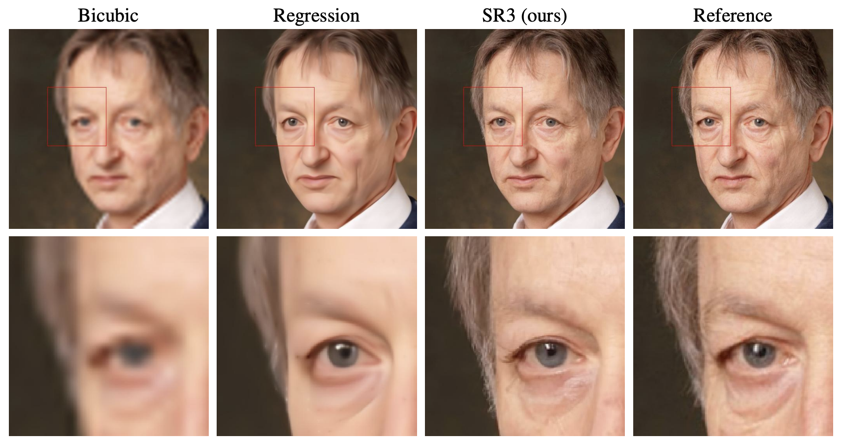
Super resolution is the process of enhancing the resolution of an image or video. The task of Super-Resolution can be defined as a mapping from \(x_{lr} \in \R^{w \times h \times c}\) to \(\hat{x}_{hr} \in \R^{\bar{w} \times \bar{h} \times c}\), where \(\bar{w} > w\) and \(\bar{h} > h\) (\(x_{hr}\) is the high-resolution image; \(x_{lr}\) is the low-resolution image; \(\hat{x}_{hr}\) is the reconstructed high-resolution image). Traditionally, increasing resolution involved simple interpolation techniques leading to blurry outcomes. However, advanced machine learning and AI, especially convolutional neural networks (CNNs), have significantly improved this field. Super resolution aims not just to upscale images, but to reconstruct high-resolution details that closely approximate true high-resolution counterparts.
 |
|---|
| Example comparing different super resolution methods (image source: [6]) |
The equation
\[\hat{x}_{hr} = SuperRes(x_{lr};\theta)\]describes the super resolution process, where the training objective is to minimize \(L(x_{hr}, \hat{x}_{hr})\). From a signal processing perspective, this problem is inherently challenging as low-resolution images lack high-frequency information expressiveness. Reconstructing a high-resolution image from a low-resolution one requires approximating these frequencies, necessitating a deep semantic understanding of the image. By leveraging patterns learned from large datasets, SR techniques can generate clear, detailed images from low-resolution inputs, finding applications in areas like satellite imagery, medical imaging, and enhancing old video footage.
Recently, with the advancement of Diffusion models in image generation task, natrually, researchers explores the intersection between super resolution with diffusion models and have shown exciting results,offering high-quality reconstructions. A notable implementation is the SR3 architecture, which this post will explore.
History of Super Resolution
Classical Techniques
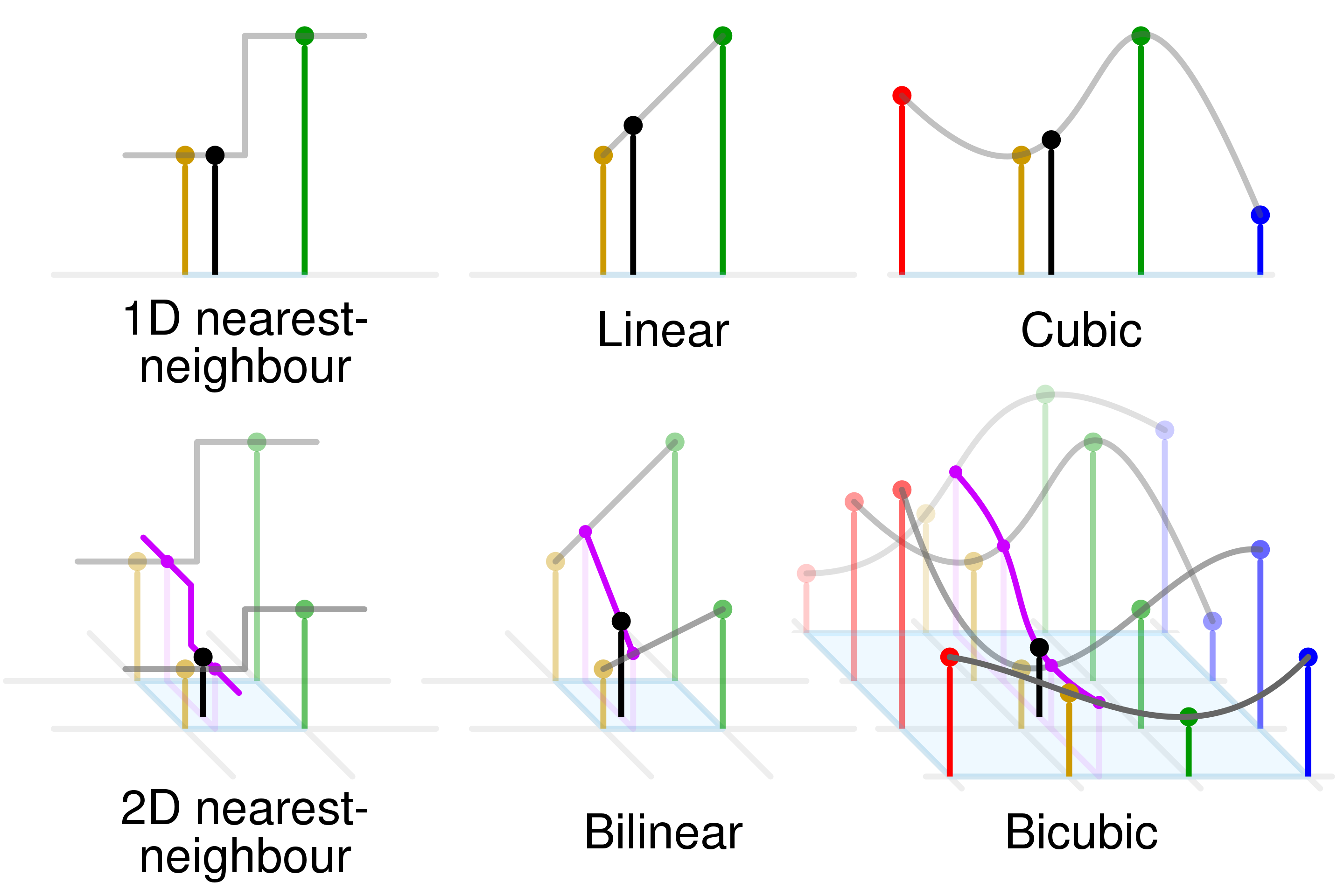
Traditional image SR methods encompass various approaches like statistical, edge-based, patch-based, prediction-based, and sparse representation techniques. These methods generate high-resolution (HR) images by utilizing the inherent information in existing pixels and image statistics. However, they often introduce noise, blur, and visual artifacts, which are significant drawbacks.
| |
|:–:|
|Different interpolation methods (image source: https://en.wikipedia.org/wiki/Bicubic_interpolation)|
|
|:–:|
|Different interpolation methods (image source: https://en.wikipedia.org/wiki/Bicubic_interpolation)|
Deep Learning Methods
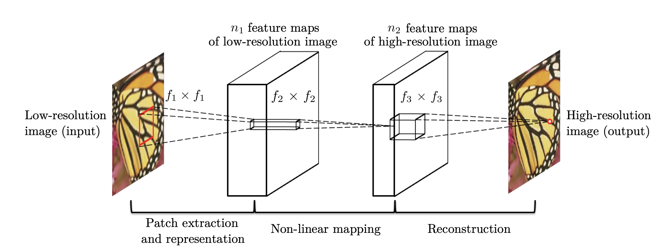
Image SR has undergone substantial improvements with the advent of Deep Learning (DL) and enhanced computational power. DL-based methods, typically employing Convolutional Neural Networks (CNNs) for direct LR to HR mapping, outperform traditional techniques. Early models like SRCNN, FSRCNN, and ESPCNN used basic CNN structures, while later developments integrated broader computer vision concepts. This includes adaptations like SRResNet from ResNet and SRDenseNet from DenseNet, incorporating residual and dense blocks, respectively. Recursive CNNs and attention mechanisms have also been integrated. DL-based SR models fall into three categories: Pixel-based, GAN-based, and Flow-based, each with distinct training objectives.
| |
|:–:|
|SRCNN architecture (image source: [2])|
|
|:–:|
|SRCNN architecture (image source: [2])|
GAN Methods
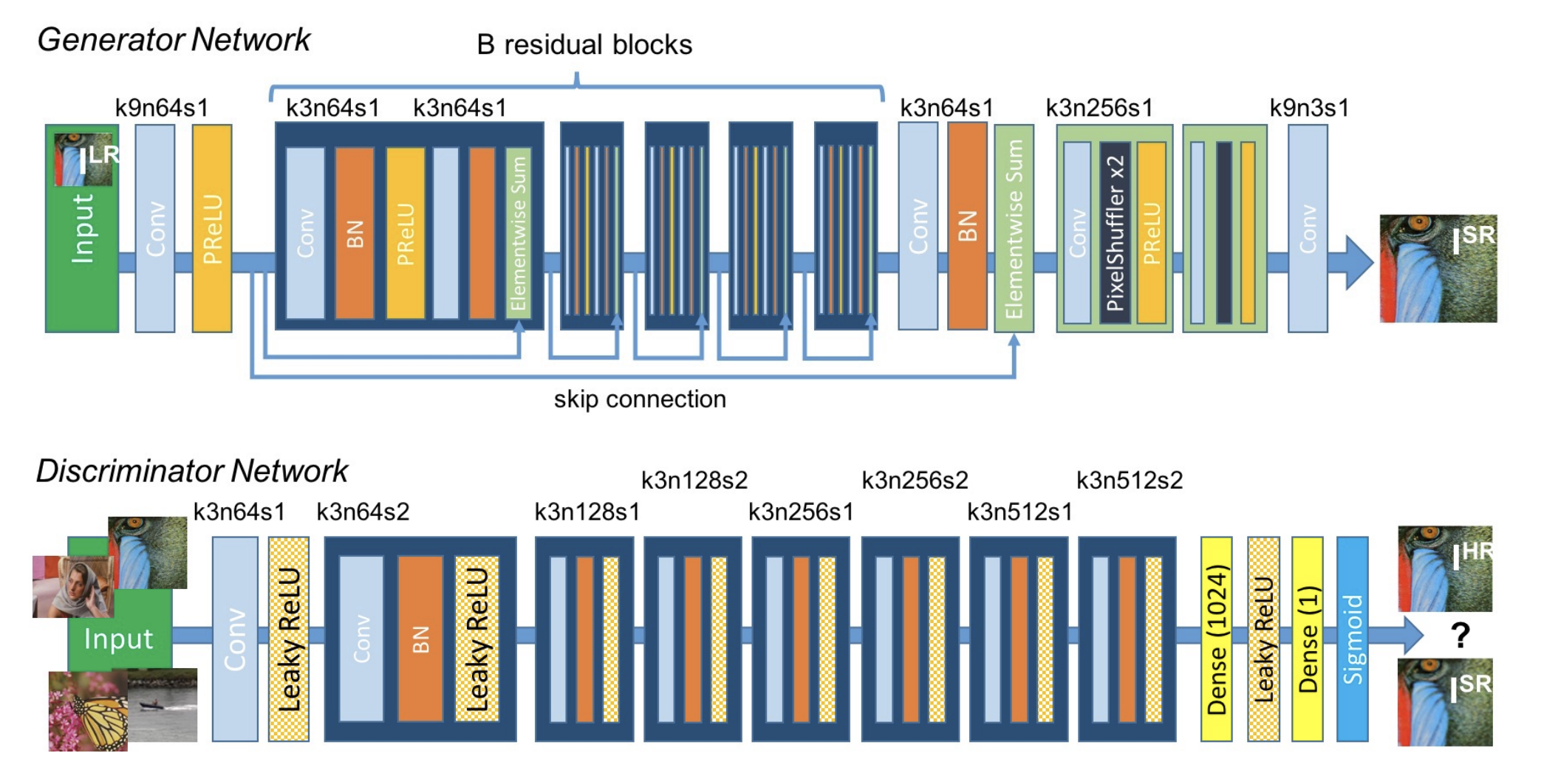
GANs operate with two CNNs - a generator and a discriminator, trained in tandem. The generator creates HR images to deceive the discriminator, which differentiates between generated and real images. Models like SRGAN and ESRGAN use a mix of adversarial and content loss to create sharper, more detailed images. Despite their ability to produce high-quality, diverse images, they face challenges like mode collapse, high computational demands, convergence issues, and require stabilization techniques.
| |
|:–:|
|SRGAN architecture (image source: [4])|
|
|:–:|
|SRGAN architecture (image source: [4])|
Flow-based Methods
These methods use optical flow algorithms to create SR images. They aim to solve the ill-posed nature of image SR by learning the conditional distribution of plausible HR images from LR inputs. Flow-based methods use a fully invertible encoder that maps HR images to a latent flow space, ensuring precise reconstruction. They are known for training stability but are computationally intensive.
Diffusion Methods
Diffusion-based methods in SR gradually transform a random distribution of pixels into a structured high-resolution (HR) image. They function by reversing a diffusion process, starting from noise and progressively refining it into a detailed image through a series of learned steps. Different from the original diffusion model introduced in DDPM, these diffusion based super resolution methods generates a high resolution image under the guidance of a lower resolution image. This approach excels in capturing fine details and textures, producing high-quality HR images that are often more realistic and less prone to artifacts compared to other methods. The focus of this post, SR3 (Image Super-Resolution via Iterative Refinement), belongs to this exciting category.
|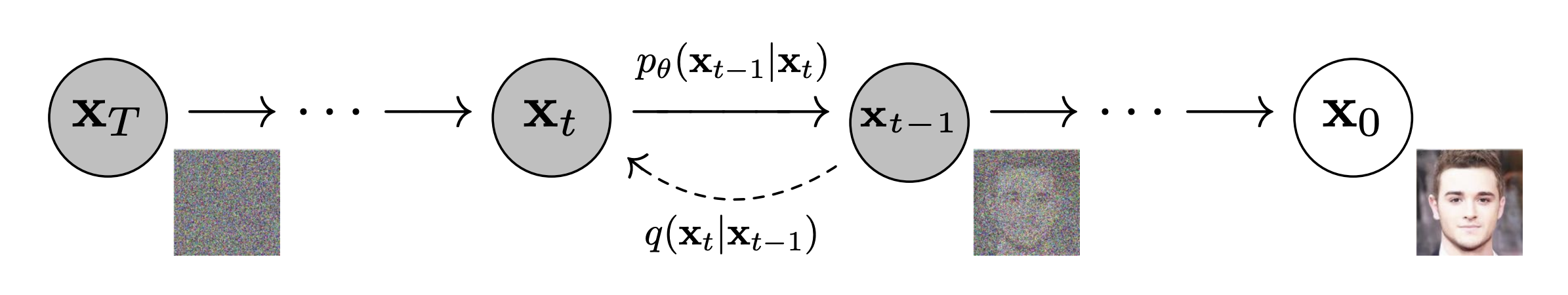 |
|:–:|
|Diffusion process (image source: [3])|
|
|:–:|
|Diffusion process (image source: [3])|
Image Super-Resolution via Iterative Refinement
Image Super-Resolution via Iterative Refinement (SR3) is a deffusion-based method that takes in a interpolated low resolution input along with random noise to generate a high resolution counter part using the diffusion model denoising process.
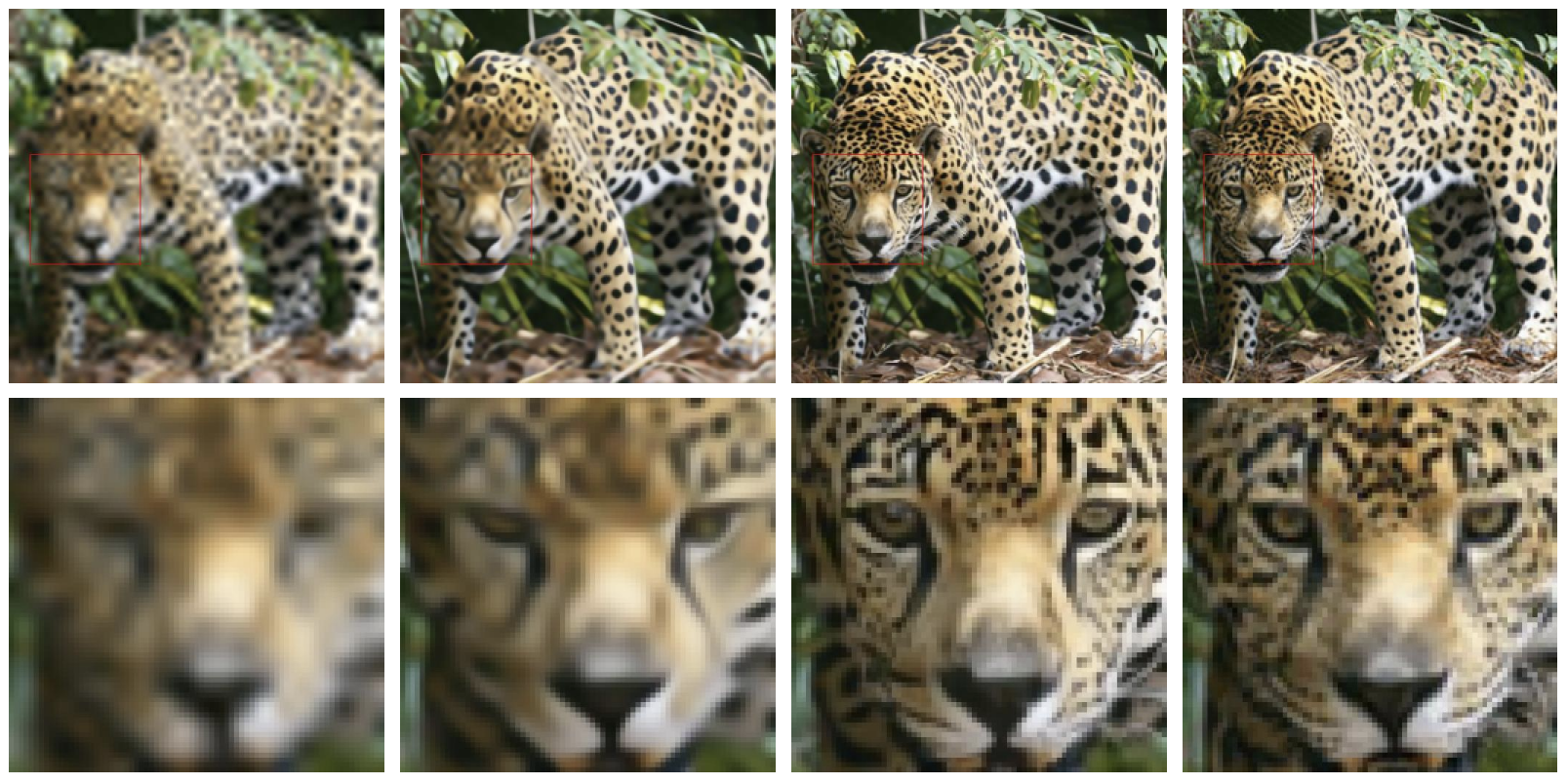 |
|---|
| example output of sr3 (image source: [6]) |
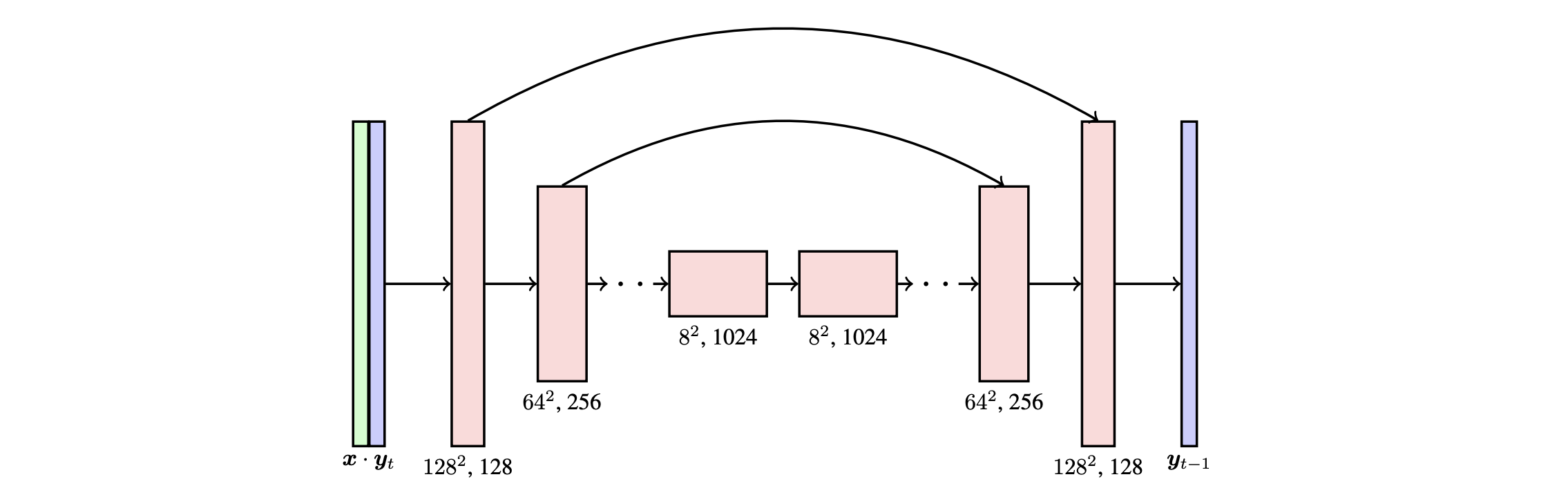
SR3 uses a similar U-net architecture to the DDMP with some improvements and adoption to suit the super resolution objective. The SR3 U-net model uses the residual block from BigGAN, which is a two-layer CNN with skip connection along with normalizations. The model uses 1.interpolated low resolution image (the paper used bicubic interpolation) to map a low resolution image to higher resolution and 2.high resolution random noise as input (concatenated on the channel dimension). And uses the U-net archietecture illistrated in Figure 3 to iteratively denoise the noisy input. Finally, the loss is calculated using l1-loss between super-resolution output and the ground-truth high resolution image \(|\hat{x}_{hr} - x_{hr}|_1\).
Pytorch Implementation
Downsample Block
The BigGAN downsample block that consists of 1. a residual path that is reduced in in the channel dimension using 1x1 conv and downsampled using average pool 2. a main path that first passes through an activation; a 3x3 conv; an activation; a 3x3 conv and an average pool for downsample. Finally the residual is added with the main path to form the final output of the downsample resblock.
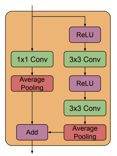 |
|---|
| BigGAN downsample resblock (used in SR3) (image source: [1]) |
class DownsampleResBlock(nn.Module):
    def __init__(self, in_channels, out_channels, time_emb_dim):
        super().__init__()
        # time embedding
        self.time_mlp = nn.Linear(time_emb_dim, in_channels)

        # Skip path layers
        self.skip_conv = nn.Conv2d(in_channels, out_channels, kernel_size=1, stride=1, padding=0)
        self.skip_avg_pool = nn.AvgPool2d(2, stride=2)

        # Main path layers
        self.conv1 = nn.Conv2d(in_channels, out_channels, kernel_size=3, stride=1, padding=1)
        self.conv2 = nn.Conv2d(out_channels, out_channels, kernel_size=3, stride=1, padding=1)
        self.avg_pool = nn.AvgPool2d(2, stride=2)

        self.relu = nn.ReLU()

    def forward(self, x, t):
        # compute time embedding
        t_emb = self.relu(self.time_mlp(t))
        t_emb = t_emb[(..., ) + (None, ) * 2]

        # Skip connection path
        skip = self.skip_conv(x)
        skip = self.skip_avg_pool(skip)

        # Main path
        x = x + t_emb
        x = self.conv1(self.relu(x))
        x = self.conv2(self.relu(x))
        x = self.avg_pool(x)

        # add the main path with the skip connection path
        out = x + torch.div(skip, math.sqrt(2))
        return out
Upsample block
The SR3 U-net model adopts the residual block used in BigGAN as a basic building block. The BigGAN resblock consists 1. a residual path that is upsampled and amplified in in the channel dimension using 1x1 conv 2. a main path, which takes-in the U-net downsample residule and concatenated on the channel dimension, that is first normalized and passed through an activation; upsampled using transposed convolution; a 3x3 conv; a normalization; an activation; finally a 3x3 conv. The two paths are added together to form the output of the upsample resblock.
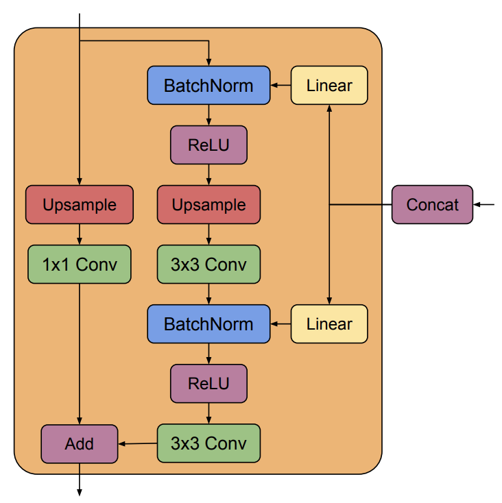 |
|---|
| BigGAN upsample resblock (used in SR3) (image source: [1]) |
class UpsampleResBlock(nn.Module):
    """
    A upsample U-Net res block.
    """

    def __init__(self, in_channels, out_channels, time_emb_dim):
        super().__init__()

        # time embedding
        self.time_mlp = nn.Linear(time_emb_dim, in_channels * 2)

        # Skip path layers
        self.skip_upsample = nn.ConvTranspose2d(in_channels, in_channels, kernel_size=2, stride=2, padding=0)
        self.skip_conv = nn.Conv2d(in_channels, out_channels, kernel_size=1, stride=1, padding=0)

        # Main path layers
        self.bn1 = nn.BatchNorm2d(in_channels * 2)
        self.upsample = nn.ConvTranspose2d(in_channels * 2, in_channels * 2, kernel_size=2, stride=2, padding=0)
        self.conv1 = nn.Conv2d(in_channels * 2, out_channels, kernel_size=3, stride=1, padding=1)
        self.bn2 = nn.BatchNorm2d(out_channels)
        self.conv2 = nn.Conv2d(out_channels, out_channels, kernel_size=3, stride=1, padding=1)

        self.relu = nn.ReLU()

    def forward(self, x, res, t):
        # compute time embedding
        t_emb = self.relu(self.time_mlp(t))
        t_emb = t_emb[(..., ) + (None, ) * 2]

        # compute skip path
        skip = self.skip_upsample(x)
        skip = self.skip_conv(skip)

        # concat the residual
        x = torch.cat([x, res], dim=1)
        # Main path
        x = x + t_emb
        x = self.relu(self.bn1(x))
        x = self.upsample(x)
        x = self.relu(self.bn2(self.conv1(x))) 1 + batchnorm + relu
        x = self.conv2(x)

        # add skip and main
        out = x + torch.div(skip, math.sqrt(2))

        return out
NOTE: The paper doesn’t explicitly specify the details of time embedding (since BigGAN doesn’t need time embedding). The current implementation injects the time embedding before the first convolution layer (same for downsample). The position of time embedding insertion is discussed more in the experiment section. Also the SR3 paper specifies that they modified the residual block to scale the residual connection by $\frac{1}{\sqrt2}$, which is reflected in the implementation.
U-net
Finally, putting everything together, we have the full u-net archietecture that is consist of the upsampling and downsampling blocks implemented above.
 |
|---|
| U-net architecture used by SR3 (image source: [6]) |
class Unet(nn.Module):
    """
    A Unet architecture.
    """

    def __init__(self, channels=1, image_size=32):
        super().__init__()
        image_channels = channels
        down_channels = (64, 128, 256, 512, 1024)
        up_channels = (1024, 512, 256, 128, 64)
        out_dim = channels
        time_emb_dim = image_size

        # Time embedding
        self.time_mlp = nn.Sequential(
            SinusoidalPositionEmbeddings(time_emb_dim),
            nn.Linear(time_emb_dim, time_emb_dim), nn.ReLU())

        # Initial projection
        self.conv0 = nn.Conv2d(2*image_channels, down_channels[0], 3, padding=1)

        # down sample blocks
        self.down_blocks = nn.ModuleList([
            DownsampleResBlock(in_ch, out_ch, image_size)
            for in_ch, out_ch in zip(down_channels[:-1], down_channels[1:])
        ])

        # up sample blocks
        self.up_blocks = nn.ModuleList([
            UpsampleResBlock(in_ch, out_ch, image_size)
            for in_ch, out_ch in zip(up_channels[:-1], up_channels[1:])
        ])

        self.output = nn.Conv2d(up_channels[-1], out_dim, 1)

    def forward(self, x, timestep):
        # Embedd time
        t = self.time_mlp(timestep)

        # Initial conv
        x = self.conv0(x)
        # Unet residuals
        residual_inputs = []

        for block in self.down_blocks:
            x = block(x, t)
            residual_inputs.append(x)


        for block, res in zip(self.up_blocks, reversed(residual_inputs)):
            x = block(x, res, t)

        return self.output(x)
Experiments
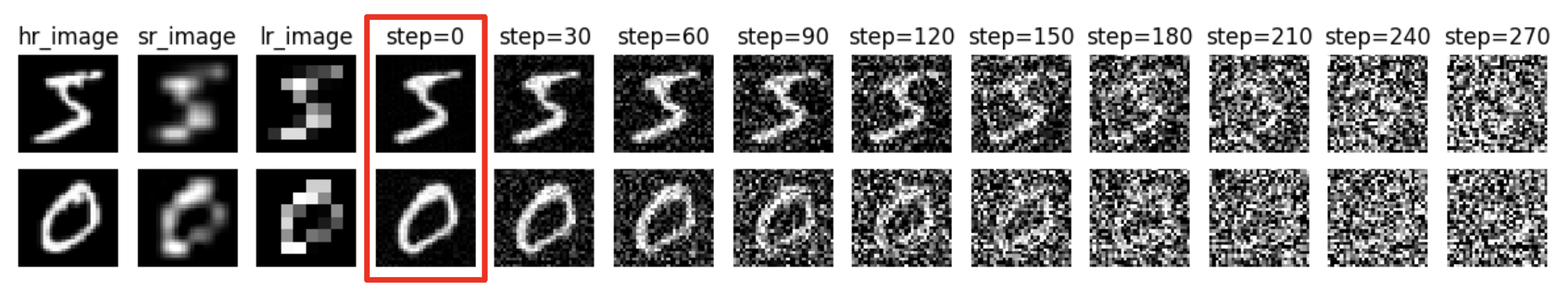
Due to resource limitions, I wasn’t able to reproduce the results discussed in the original paper, which was trained on the Flickr-Faces-HQ and ImageNet 1K datasets. Instead, I experimented with two smaller datasets: MNIST and MiniPlaces. For MNIST, I trained a model that produce super-resolution at 8x8 -> 32x32. For MiniPlaces I trained a model that produce super-resolution at 32x32 -> 128x128.
For the two datasets, the images are first downsampled using bilinear interpolation to get $x_{lr}$ (the low resolution image) and then upscaled using the same method to get $\hat{x}_{hr}$ (interpolated high resolution image). These pairs of images serves as the training input and ground-truth.
Before training the SR3 U-net model, I trained a simple U-net model using the implementation from Assigment 4. Below is some brief results that showed very good performance after 5 epochs of training.
 |
|  |
:—————————————: |
| Super-Resolution output on the MNIST dataset. (hr_image -> reference, lr_image -> downsampled image, sr_image -> bicubic interpolation, step = 0 -> model output) |
|
:—————————————: |
| Super-Resolution output on the MNIST dataset. (hr_image -> reference, lr_image -> downsampled image, sr_image -> bicubic interpolation, step = 0 -> model output) |
Compared to the interpolated high resolution image, the model output indeed has more details and have more defined edges.
As noted previously, the SR3 paper doesn’t explicitly specify the location of which the time embedding is inserted into the BigGAN residual block and the original implementation has no notion of time. Yet, as a essential part of diffusion model, time embedding is a necesity for good model performance. Thus I experimented with the time embedding injection locations (1. before first conv layer 2. between first and second conv layer 3. after the conv layers) within the residual block and observed that time embedding inserted before the first convolution layer seems to work the best (details can be found in jupyter notebook). Thus in my final model implementation I choose to do the element-wise sum of the time embedding before the first convolution layer for both upsampling and downsampling blocks.
|  |
| :—————————————————————————————————————————————————————: |
| Super-Resolution output on the MNIST dataset. (hr_image -> reference, lr_image -> downsampled image, sr_image -> bicubic interpolation, step = 0 -> model output) |
|
| :—————————————————————————————————————————————————————: |
| Super-Resolution output on the MNIST dataset. (hr_image -> reference, lr_image -> downsampled image, sr_image -> bicubic interpolation, step = 0 -> model output) |
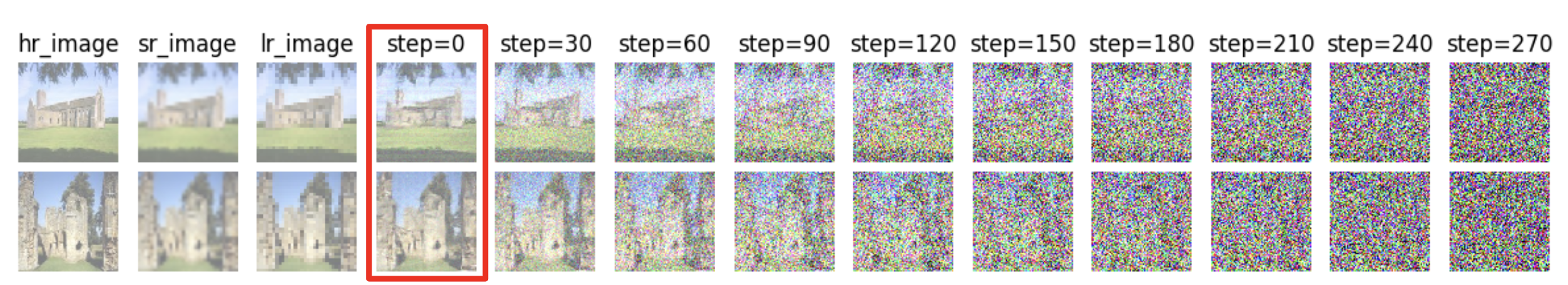
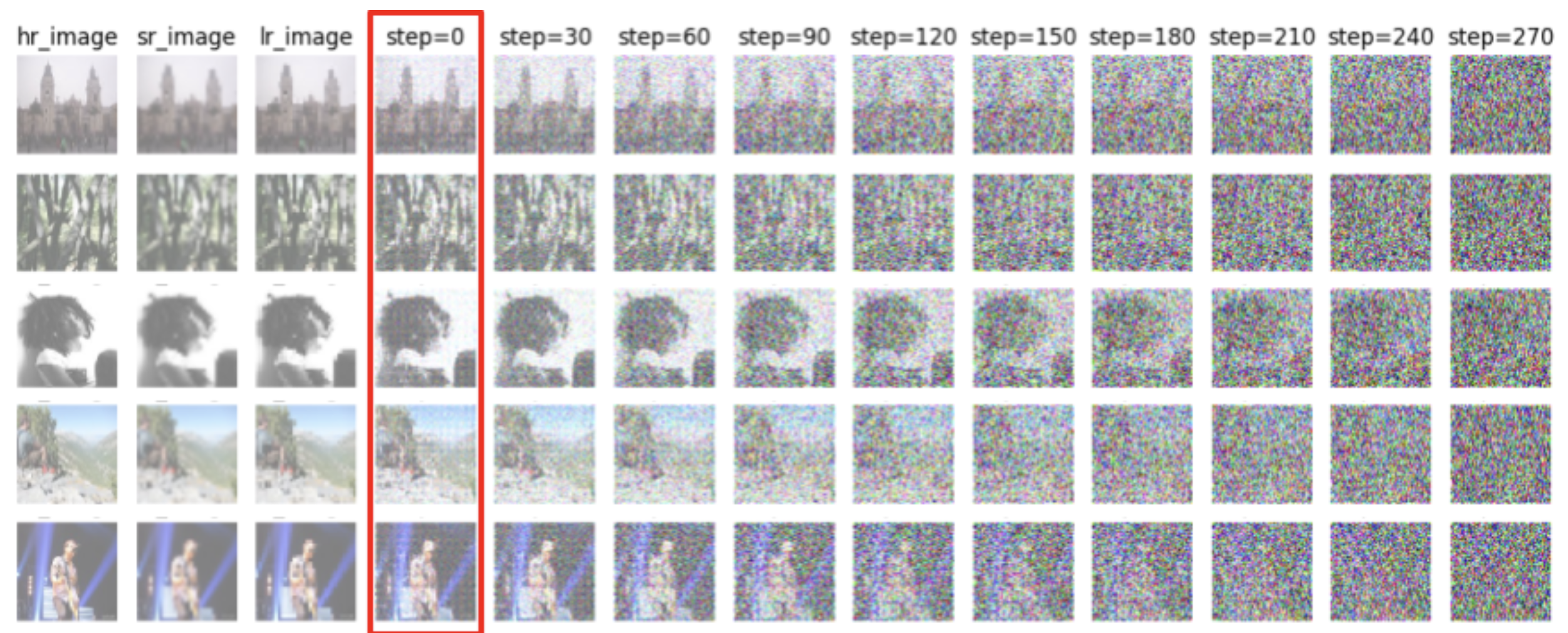 |
|---|
| Super-Resolution output on the MiniPlaces dataset. (hr_image -> reference, lr_image -> downsampled image, sr_image -> bicubic interpolation, step = 0 -> model output) |
The above figure is the testing result of super-resolution model using SR3 U-net architecture after 5 epochs of training. The left most column is the reference images (original high resolution image); the second column is the interpolated image from low resolution; the third column is the low resolution image; the fourth column is the reconstructed high resolution image by the model. The result from the MNIST super resolution experiment shows promising results. As we can observe, the model is able to reconstruct a high resolution quality image from the downsampled low resolution image. On the other hand, the model doesn’t perform as well on the MiniPlaces dataset after 5 epochs. Although comparing to the interpolated image, the output images still captures more details and have sharper edges, the output images is still somewhat noisy.
NOTE: the authors of SR3 mentions the limitations of current super resolution criterions and uses human evaluation instead, so I will just present the results without analyzing it quantitatively.
Conclusion
In conclusion, this comprehensive exploration into the realm of super-resolution, particularly through the lens of diffusion models, represents a significant leap in our ability to enhance image quality. By delving into the historical context and evolution of super-resolution methods, from classical techniques to advanced diffusion methods like SR3, this post underscores the remarkable progress in image processing. The practical implementation using a PyTorch-based U-net architecture, adapted from BigGAN and tailored for SR3, illustrates the practical applicability of these concepts. The experiments with datasets like MNIST and MiniPlaces demonstrate the ability of these methods in producing high-resolution images with more defined edges and details compared to traditional interpolation techniques. Although quantitative analysis is not the focus here, the visual results speak volumes about the potential of diffusion models in super-resolution tasks. This exploration not only provides a deep understanding of the current state-of-the-art techniques in image super-resolution but also sets the stage for future advancements in this exciting field.
Papers mentioned
[1] Brock, Andrew. et al. “Large Scale GAN Training for High Fidelity Natural Image Synthesis.” arXiv:1809.11096 (2018).
[2] Dong, Chao. et al. “Image Super-Resolution Using Deep Convolutional Networks.” arXiv:1501.00092 (2015).
[3] Ho, Jonathan. et al. “Denoising Diffusion Probabilistic Models.” arXiv:2006.11239 (2020).
[4] Ledig, Christian. et al. “Photo-Realistic Single Image Super-Resolution Using a Generative Adversarial Network.” arXiv:1609.04802 (2016).
[5] Moser, Brian B. et al. “Diffusion Models, Image Super-Resolution And Everything: A Survey.” arXiv:2401.00736 (2024).
[6] Saharia, Chitwan. et al. “Image Super-Resolution via Iterative Refinement.” arXiv preprint arXiv:2104.07636 (2021).