Hierarchical Label Explainability

Understanding how hierarchical labels affect saliency maps can unlock new pathways for model transparency and interpretability. This post explores the motivation, existing methods, and implementation of our project on hierarchical label explainability.

• Introduction
• Motivation
• Exisitng Methods
  • Saliency Maps
  • Label Granularity and Accuracy
• Our Project
  • Starter Code
  • Dataset
  • Implementation
• Experiements
• Results and Observations
  • Model Accuracy:
  • Saliency Maps:
  • Additional Observations:
  • Challenges and Limitations:
• Conclusion and Future Work
• Reference

Introduction

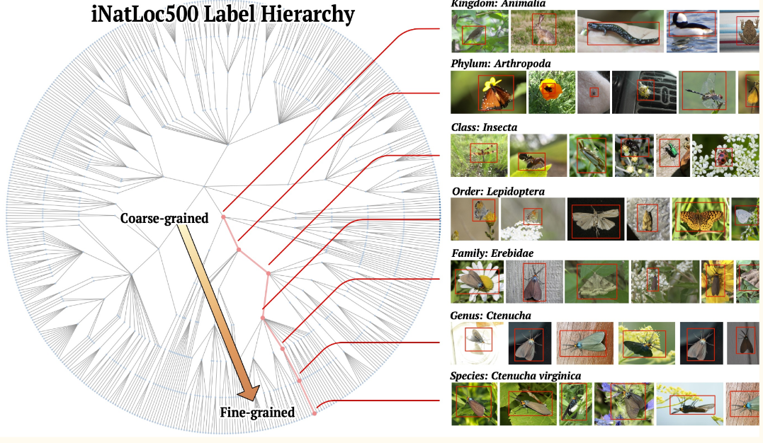
Deep learning models often operate as black boxes, making their decisions difficult to interpret. Saliency maps, which highlight areas of an image contributing most to a model’s decision, are a key tool for visualization. By studying how saliency maps change across levels of abstraction in hierarchical labels, we aim to enhance interpretability and provide finer-grained insights into model behavior. Our focus is on the iNatLoc500 dataset, a challenging benchmark with 500 species organized in a label hierarchy.

Motivation

Model transparency is crucial for trust and accountability in AI systems. Details, such as whether a model correctly distinguishes between closely related categories (e.g., Bulldog and Husky), can reveal its true understanding. Hierarchical labeling offers a structured approach to interpretability, breaking down decisions into different levels of granularity. This project seeks to address:

How hierarchical labels influence saliency maps.
Whether these insights improve model transparency and user trust.

Exisitng Methods

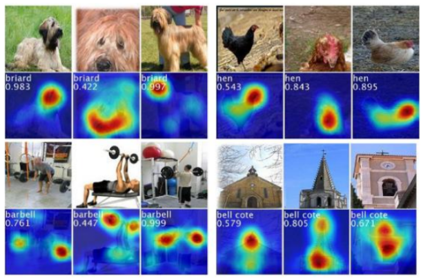
Saliency Maps

Saliency maps highlight the regions in an input image that contribute most to the model’s predictions. Areas with high brightness correspond to influential regions. Saliency is computed using gradients of the model’s output with respect to input pixels

Key References: [1] Simonyan et al. (2014): Introduced visualization techniques for convolutional networks.
[2] Samek et al. (2015): Evaluated methods for visualizing learned features in deep networks.

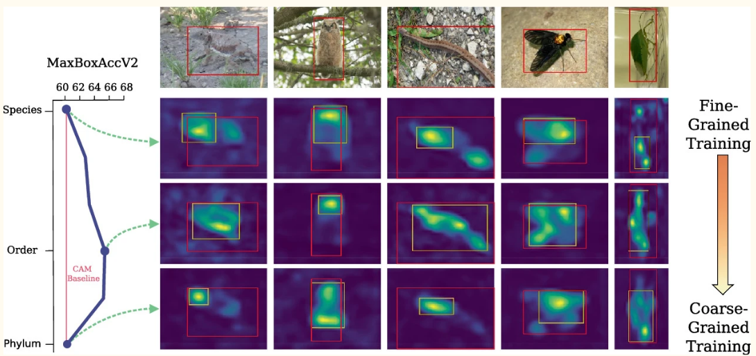
Label Granularity and Accuracy

A study by Cole et al. (2022) investigated how hierarchical labeling affects accuracy. Using ResNet50 and iNatLoc500, they demonstrated the potential for granularity to improve interpretability. However, their implementation lacked accessible code, highlighting a gap we aim to address.

Our Project

Starter Code

To start the project, we found an existing project that worked on the classification of birds within the iNatLoc500 dataset. The existing codebase (https://www.kaggle.com/code/sharansmenon/inaturalist-birds-pytorch), made use of efficientnet and resnet architectures to classify the birds. We used this codebase as a starting point to implement our project.

Dataset

The input dataset (https://www.kaggle.com/datasets/sharansmenon/inat2021birds) to the model consisted of 74k images of birds, consisting of 1486 bird species. The model takes 10% of the images as validation, 10% as test, and the remaining 80% as training data. The model was trained for 14 epochs. The model was trained using the Adam optimizer with a learning rate of 0.001.

Below are a few example images of the input:

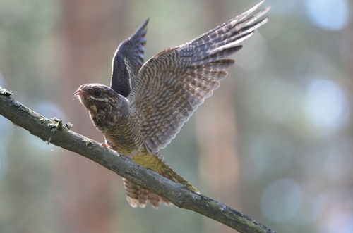
Each image is annotated with a hierachical label linked to their taxonomic classification. The labels are structured in a hierarchy, with each label representing a different level of granularity. Some examples of these are shown below:

03114_Animalia_Chordata_Aves_Accipitriformes_Accipitridae_Accipiter_nisus
03124_Animalia_Chordata_Aves_Accipitriformes_Accipitridae_Buteo_albonotatus
03167_Animalia_Chordata_Aves_Accipitriformes_Accipitridae_Ictinia_mississippiensis

The labels are structured in the following way:

{ID}_{Kingdom}_{Phylum}_{Class}_{Order}_{Family}_{Genus}_{species}

In our project, the plan was to run two experiments, where we run the model on the dataset, with the “species” level of granularity, and then run it again to train it on the “Family” level of granularity. We then planned to generate CAMs for the model and compare the results, seeing how the model performed at different levels of granularity, and visually inspecting how the CAMs changed based on the level of granularity.

Implementation

First running an existing codebase, we then implemented our own ideas to experiment with the concept of Abstracted Labels and Saliency Maps. We implemented a few features to the existing codebase to generate CAMs and abstract the labels of the birds into their respective families. These steps are described below:

1. CAM Mapping Computation:

Computed Class Activation Maps (CAM) to visualize the most discriminative regions of the image for each class. We added the following set of code to the existing codebase to generate CAMs for the model. We made use of the pytorch-grad-cam library to generate the CAMs. The code below shows how to generate CAMs for a given model and input image.

from pytorch_grad_cam import GradCAM
from pytorch_grad_cam.utils.model_targets import ClassifierOutputTarget
from pytorch_grad_cam.utils.image import show_cam_on_image
import matplotlib.pyplot as plt

# Ensure the model is in evaluation mode
model.eval()

# Get a single data sample from the test loader
data, target = next(iter(test_loader))
data = data[:1]
data = data.to(device)
data.requires_grad = True  # Ensure gradients are tracked

# Specify the target layer
target_layer = model.blocks[-1][-1].conv_pwl  # Adjust based on your model architecture

# Initialize GradCAM
cam = GradCAM(model=model, target_layers=[target_layer])

# Specify the class index (e.g., 0) to compute CAM for
class_index = 0  # Replace with your desired class index
targets = [ClassifierOutputTarget(class_index)]

# Generate the CAM
grayscale_cam = cam(input_tensor=data, targets=targets)
grayscale_cam = grayscale_cam[0, :]  # Select the first batch element

# Overlay CAM on the input image
input_image = data[0].permute(1, 2, 0).cpu().detach().numpy()  # Adjust if necessary
input_image_normalized = (input_image - input_image.min()) / (input_image.max() - input_image.min())
cam_image = show_cam_on_image(input_image_normalized, grayscale_cam, use_rgb=True)

# Display the CAM
plt.imshow(cam_image)
plt.axis('off')
plt.show()

2. Class Abstraction:

In the dataset, each bird is labelled in a hierachical fashion, this meant that birds of the same “Family” could be grouped into the same class. We did this by developing a custom dataloader that grouped the birds into their respective families. The code below shows how we implemented this:

class CustomImageFolder(ImageFolder):
    def find_classes(self, directory):
        # Get all original folder names
        original_classes = sorted(entry.name for entry in os.scandir(directory) if entry.is_dir())
        # Generate processed class names
        processed_classes = ['_'.join(cls.split('_')[2:-2]) for cls in original_classes]
        # Deduplicate processed class names in case of overlaps
        processed_classes = sorted(set(processed_classes))

        # Map processed class names to indices
        class_to_idx = {cls: i for i, cls in enumerate(processed_classes)}

        # Create a reverse map for original class names to processed class indices
        original_to_processed_idx = {
            original: class_to_idx['_'.join(original.split('_')[2:-2])] for original in original_classes
        }

        # Store the mapping internally
        self.original_to_processed_idx = original_to_processed_idx
        self.classes = processed_classes  # Override to use processed class names
        return processed_classes, class_to_idx

    def __getitem__(self, index):
        # Default behavior: get image tensor and original integer label
        sample, original_target = super().__getitem__(index)
        # Map original target to processed class index
        processed_target = self.original_to_processed_idx[self.classes[original_target]]
        return sample, torch.tensor(processed_target)

3. Training:

The rest of the code was kept largely the same, the original model provided various standard techniques for improving accuracy, prominently including data augmentation, as shown in the following snippet:

def get_data_loaders(data_dir, batch_size, train=False):
    if train:
        transform = transforms.Compose([
            transforms.RandomHorizontalFlip(p=0.5),
            transforms.RandomVerticalFlip(p=0.5),
            transforms.RandomApply(torch.nn.ModuleList([transforms.ColorJitter()]), p=0.1),
            transforms.Resize(256),
            transforms.CenterCrop(224),
            transforms.ToTensor(),
            transforms.Normalize((0.485, 0.456, 0.406), (0.229, 0.224, 0.225)),
            transforms.RandomErasing(p=0.2, value='random')
        ])
        all_data = CustomImageFolder(data_dir + "/bird_train", transform=transform)
        train_data_len = int(len(all_data) * 0.78)
        valid_data_len = int((len(all_data) - train_data_len) / 2)
        test_data_len = len(all_data) - train_data_len - valid_data_len
        train_data, val_data, test_data = random_split(all_data, [train_data_len, valid_data_len, test_data_len])
        train_loader = DataLoader(train_data, batch_size=batch_size, shuffle=True, num_workers=4)
        return train_loader, train_data_len

    else:
        transform = transforms.Compose([
            transforms.Resize(256),
            transforms.CenterCrop(224),
            transforms.ToTensor(),
            transforms.Normalize((0.485, 0.456, 0.406), (0.229, 0.224, 0.225))
        ])
        all_data = CustomImageFolder(data_dir, transform=transform)
        train_data_len = int(len(all_data) * 0.78)
        valid_data_len = int((len(all_data) - train_data_len) / 2)
        test_data_len = len(all_data) - train_data_len - valid_data_len
        train_data, val_data, test_data = random_split(all_data, [train_data_len, valid_data_len, test_data_len])
        val_loader = DataLoader(val_data, batch_size=batch_size, shuffle=True, num_workers=4)
        test_loader = DataLoader(test_data, batch_size=batch_size, shuffle=True, num_workers=4)
        return val_loader, test_loader, valid_data_len, test_data_len

The rest of the code used in this project can be found in the notebook found at: https://drive.google.com/file/d/12CoaUaMKL7c3gHc3z8qx8P1891WXERlW/view?usp=sharing

Experiements

The experiments of the project essentially consisted of two parts, the first was to apply CAMs to the existing code (trained on the “species” level of granularity) and generate CAMs for the model. The second part was to adapt the code and to train the model on the “Family” level of granularity and generate CAMs for the model. We then compared 1) the accuracy of the model at the two levels of granularity and 2) the CAMs generated by the model at the two levels of granularity.

Results and Observations

Model Accuracy:

Although the accuracy wasn’t the focus of the model, we thought it interesting to investigate how the model performed at the two levels of granularity. The model trained on the “species” level of granularity achieved a validation accuracy of 0.80 with 14 epochs of training, which is a relatively good result.

Due to constrained compute resources, we were unable to train the model on the “Family” level of granularity for the same number of epochs. However, the model achieved a validation accuracy of 0.67 after 5 epochs of training, while the “Species” model’s accuracy at this point was only 0.56. This suggests that training on the “Family” level of granularity performs better than training on the “Species” level of granularity. There are a few possible reasons for this.

Since the “Family” model combines images and training examples across several species, it receives a higher number of training examples per class, which could lead to better generalization.

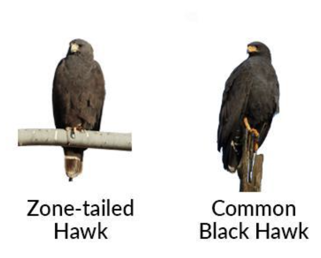
Humans often find it is easier to distinguish between birds of the different “Family” level of granularity over different “Species” due to the more obvious generally shared features of birds within the same family. For example, most people can distinguish between a hawk and a dove, but most will have a more difficult time distinguishing between a “Zone-tailed Hawk” and a “Common Black Hawk”. With the “Family” model performing better than the “Species” model, our results support this from the perspective of the model.

Saliency Maps:

CAMs were generated for the “Species” and “Family” models. We visually compared several examples, to see the differences in what they represented. Unfortunately, due to the batching strategy we used to to load the data and train, it made it difficult to feed the same images into the either model (when we combined subsets into Families, it made it difficult to retrieve the same image as input into the CAM generator). This is an issue that we would like to address in future work.

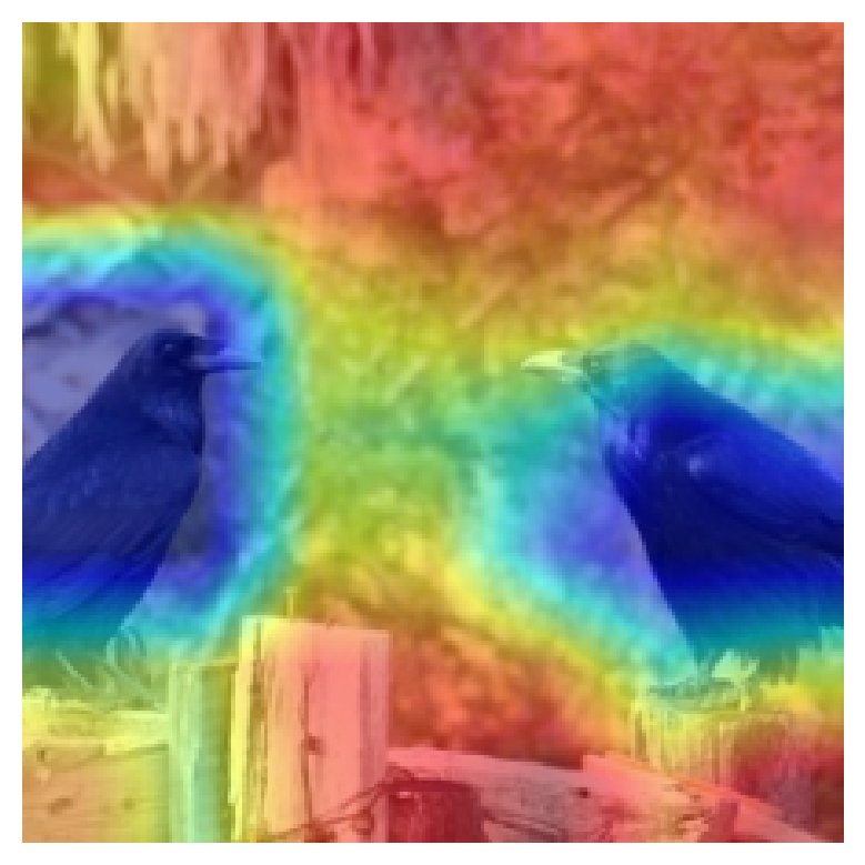
However, even just considering the CAMs we generated for either model, it is very clear that providing differing granularities leads the model to focus on different parts of the image. Shown below are a few examples of the saliency maps generated for the “Species” and “Family” models.

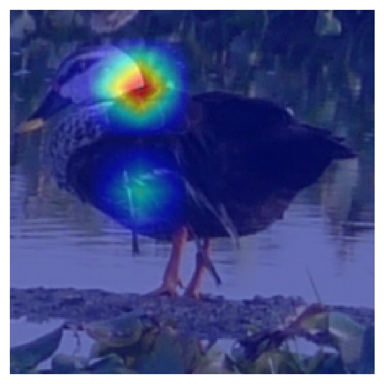
Species Model:

Family Model:

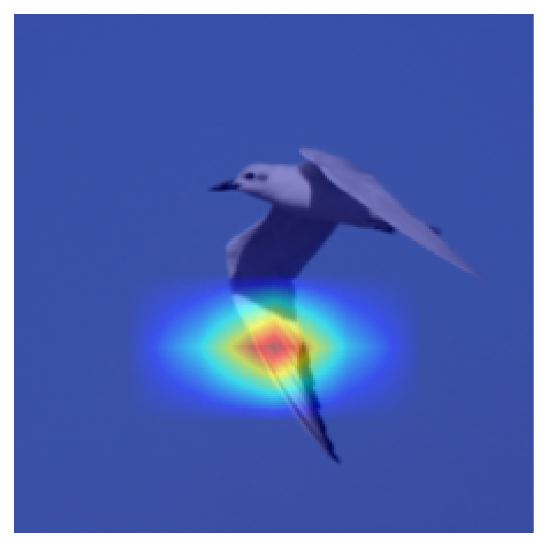
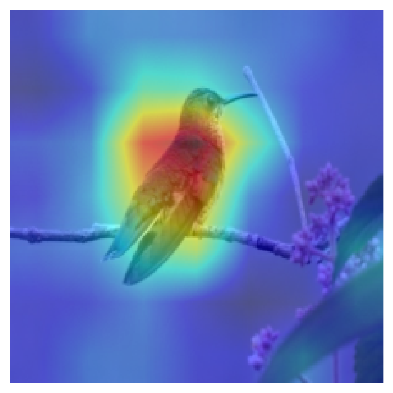
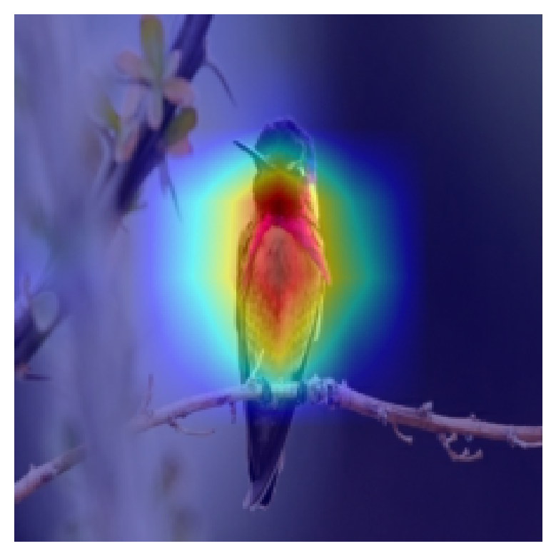
From the above images, it is clear that the “Species” model focusses more on specific parts of the bird (such as the neck and wing in the first “Species” image, and the tail in the second one), while the “Family” model looks at the whole bird, and the surrounding context much more (as evidenced by the second two “Family” model images, focussing on the entire bird shape). The first image of the “Family” also points to a characterstic part of “Seagull” - the wing. This is interesting, and in line with the way that humans interpret and classify bird species and families.

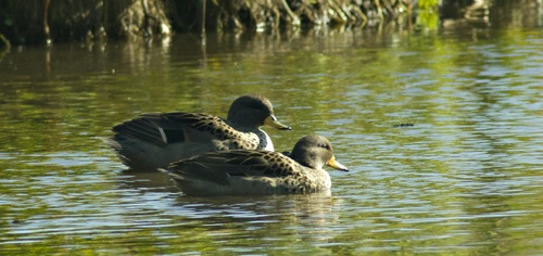
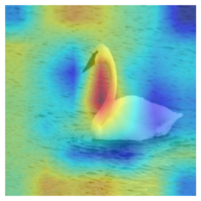
Additional Observations:

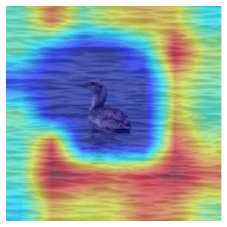
It was interesting to note, that he “Family” model, also takes the environment the bird is in into account. For example, in the image of a swan below, the CAM highlights the water surrounding the swan, indicating that to get the correct “Family” classification, the water was a key clue for the model.

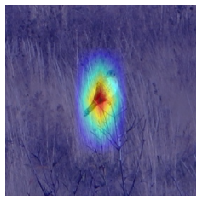
Challenges and Limitations:

Although the results are promising, there are a few limitations to the work we have done. Not every saliency map generated a result that was logically coherent with human interperatability. It is possibel that this is due to an error in our implementation, or that these examples came from a poorly represented class. This is shown in the following image, we see that the CAM is focussing on parts of the image not relevant to the bird at all - the tree background, or just the water.

This is something that could be addressed and investigated further in Future work and links with another limitation of this study. The work done here is a very high-level human-interpretation focussed overview of the effect of label granularity in Saliency mapping. A more data-focussed approach would be useful to see how much these results and thinking can be generalised to other datasets and models. The way to do this could be to generate many images, and organize them into “coherent” and “non-coherent” represntations, where the effectiveness in using the CAMs to interpret the model’s decisions can be quantified.

Conclusion and Future Work

This project demonstrated the potential of hierarchical labels to enhance interpretability through saliency maps. However, challenges remain in scaling this approach to larger datasets and improving its robustness for similar categories. Future steps include:

• Providing a more data focussed approach to quantify the problem (as described above)
• Incorporating multi-grained descriptors as suggested by Wang et al. (2015). The idea with this is to use multiple levels of granularity to improve the model’s performance and interpretability. Work has already been done towards this but would be interesting to investigate with this context
• Testing additional architectures like ResNet50 for performance comparisons.

Ultimately this framework provides some fascinating opportunities to both improve model performance and interpretability, but also in understanding the natural world. Consdering these maps it is reasonable to image that people could learn what parts of an image indicate a particular label, which could lead to more robust taxonomic classification systems. For example, by seeing how the CAMs highlight certain parts of a particular species’ wing, we could learn that this is a key feature of that species. This could be used to improve the accuracy of bird classification systems, and a similar approach could be used in other fields such as medical imaging.

Reference

[1] Simonyan, K., Vedaldi, A., & Zisserman, A. (2014). Deep Inside Convolutional Networks: Visualising Image Classification Models and Saliency Maps. arXiv preprint arXiv:1312.6034.
[2] Samek, W., Binder, A., Montavon, G., Bach, S., & Müller, K.-R. (2015). Evaluating the Visualization of What a Deep Neural Network Has Learned. arXiv preprint arXiv:1509.06321.
[3] Zhang, Q., Wu, Y. N., & Zhu, S.-C. (2018). Interpretable Convolutional Neural Networks. arXiv preprint arXiv:1710.00935.
[4] Cole, E. et al. (2022). On Label Granularity and Object Localization. In: Avidan, S., Brostow, G., Cissé, M., Farinella, G.M., Hassner, T. (eds) Computer Vision – ECCV 2022. ECCV 2022. Lecture Notes in Computer Science, vol 13670. Springer, Cham. https://doi.org/10.1007/978-3-031-20080-9_35
[5] Wang, Dequan & Shen, Zhiqiang & Shao, Jie & Zhang, Wei & Xue, Xiangyang & Zhang, Zheng. (2015). Multiple Granularity Descriptors for Fine-Grained Categorization. 2399-2406. 10.1109/ICCV.2015.276.
[6] “Hawk,” Animal Spot, https://www.animalspot.net/hawk. Accessed: Dec. 13, 2024.
—