This block is a brief introduction of your project. You can put your abstract here or any headers you want the readers to know.

Content-Based Image Retrieval: A Deep Dive

Content-Based Image Retrieval: A Deep Dive

Authors: Aral Muftuoglu, Azad Azargushasb, Vikram Chilkunda

Introduction

Content-Based Image Retrieval (CBIR) leverages mathematical representations of image content to identify visually similar images within large datasets. The process involves mapping an image, represented as a matrix of pixel intensities, into a high-dimensional feature vector space. Let \(\Phi\) represent the feature extraction function, mapping an input image \(I \in \mathbb{R}^{C \times W \times H}\) (channels, width, height) to a feature vector \(\mathbf{v} \in \mathbb{R}^D\):

\[\mathbf{v} = \Phi(I), \quad \text{where } \Phi : \mathbb{R}^{C \times W \times H} \to \mathbb{R}^D.\]

Then, we input an image to the system with the goal of retrieving similar images. To do so, the system computes a similarity score between the query image’s feature vector and those in the database using distance metrics, such as cosine similarity, Euclidean distance, or a variety of others not displayed here:

\[d(\mathbf{v}_q, \mathbf{v}_i) = \| \mathbf{v}_q - \mathbf{v}_i \|_2, \quad \text{or } \frac{\mathbf{v}_q \cdot \mathbf{v}_i}{\| \mathbf{v}_q \| \| \mathbf{v}_i \|}.\]

The top-(k) images with the highest similarity scores are returned as results, offering both visual and semantic relevance.

A query image on the left, along with two possible images retrieved on the right.

Real-World Applications

Search Engines: Google and Bing offer “Search by Image” functionalities.
E-Commerce: Platforms like Amazon and eBay enable product searches using images.

Approaches and Techniques to Image Retrieval

CBIR systems utilize various strategies to identify similar images, but follow the same pattern of extracting a meaningful representation of an image into a high-dimensional vector, and then comparing this vector to other feature vectors of images:

1. Basic Feature Extraction with CNNs

Process

The database of feature vectors is formed by sending training images through a Convolutional Neural Networks (CNNs), which extracts deep features like edges, textures, shapes, and spatial patterns. However, we skip the last (fully connected) layer to obtain a high-dimensional vector containing rich information about the image. There are many methods of storing these feature vectors in a memory-efficient way, as storing tensors with thousands of elements can occupy excessive amounts of memory, often more than available. Some such methods include vector quantization or Principal Component Analysis (PCA), which both attempt to reduce the dimensionality of the vectors while still maintaining the rich meaning encoded within.

When given a query image, we run it through the same CNN and obtain a feature vector describing the query image. Using one of several distance metrics, often cosine similarity or Euclidean distance, we find the top-k similar vectors, and return the associated images.

Feature Vectors

High-dimensional vectors (e.g., 512 or 1024 dimensions) are generated from intermediate CNN layers to represent an image, and an example feature vector from ResNet-18 is shown below:

[0.45, -0.12, 0.34, ..., 0.89]  # Image 1 (dog)
[0.47, -0.10, 0.31, ..., 0.87]  # Image 2 (dog)

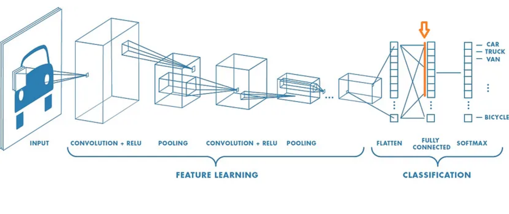
Resnet18 Architecture. The orange arrow indicates where the feature vector is extracted from the network. (image source: [1])

2: LoFTR: Detector-Free Local Feature Matching with Transformers

Motivation

LoFTR introduces a new approach to image feature detection to address challenges faced by traditional methods, such as:

Poor repeatability in low-texture areas.
Errors in repetitive patterns.
Variations in viewpoint and lighting.

LoFTR utilizes a detector-free dense matching pipeline with Transformers, diverging from traditional local feature-matching methods that rely on sequential steps: feature detection, description, and matching.
Instead, LoFTR:

Produces dense matches in regions where traditional feature detectors struggle.
Refines these matches at the coarse dense level to resolve ambiguities.

Techniques

The researchers trained two specific models for different environments:

Indoor Model: Trained on the ScanNet dataset.
Outdoor Model: Trained on the MegaDepth public dataset.

Architecture

The LoFTR architecture comprises four key components to achieve robust local feature matching:

Feature Extraction Backbone:
- Uses a standard Convolutional Neural Network (CNN) to extract multi-level features from input images.
- Generates coarse-level and fine-level features.
- Downsampling in CNN reduces input length, lowering computational costs.
Coarse-Level Feature Transformation:
- Reshapes features into 1D vectors and adds positional encodings.
- Processes features through a Transformer module, combining:
  - Self-Attention Layers: For capturing global context.
  - Cross-Attention Layers: For position-aware descriptors.
Matching Module:
- Uses a differentiable matching layer to compute a confidence matrix, identifying likely correspondences between the feature maps of two images.
- Matches are selected based on:
  - Mutual-Nearest-Neighbor Criteria.
  - A confidence threshold.
- This forms the initial set of coarse-level matches.
Fine-Level Refinement Module:
- Crops a small window around each coarse match.
- Refines these matches to produce final matches with sub-pixel accuracy.

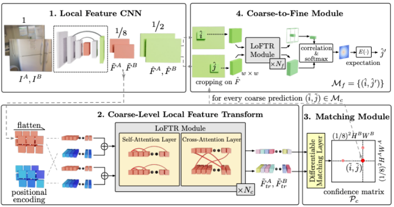
Image of the LoFTR architecture(image source: [2])

Results

LoFTR was evaluated in both indoor and outdoor environments, outperforming existing methods:

Compared to SuperGlue and DRC-Net, LoFTR produced:
- More correct matches.
- Fewer mismatches.
Delivered high-quality matches in challenging areas, such as:
- Texture-less walls.
- Floors with repetitive patterns.
Achieved first-place rankings on two public benchmarks for visual localization.

LoFTR’s results demonstrate its effectiveness in real-world applications and its reliability in addressing areas where traditional methods struggle.

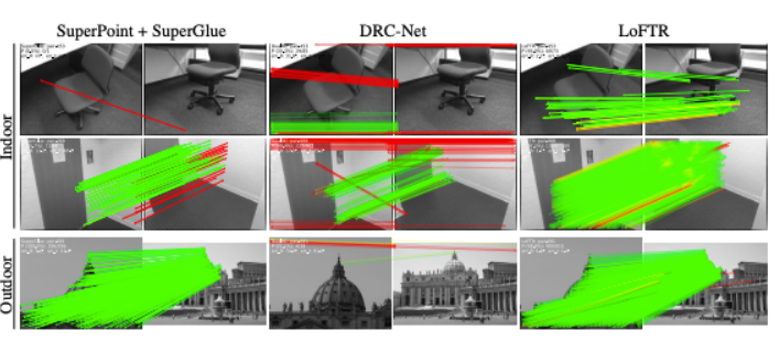
Results comparing LoTFR to other models (image source: [1])

Note: Red lines represent epipolar line errors greater than (5 \times 10^{-4}).

Attached here is our codebase implementation in Google Colab.

Implementation and Results

Let’s demonstrate our implementation using two photos of a desktop setup taken from slightly different angles:

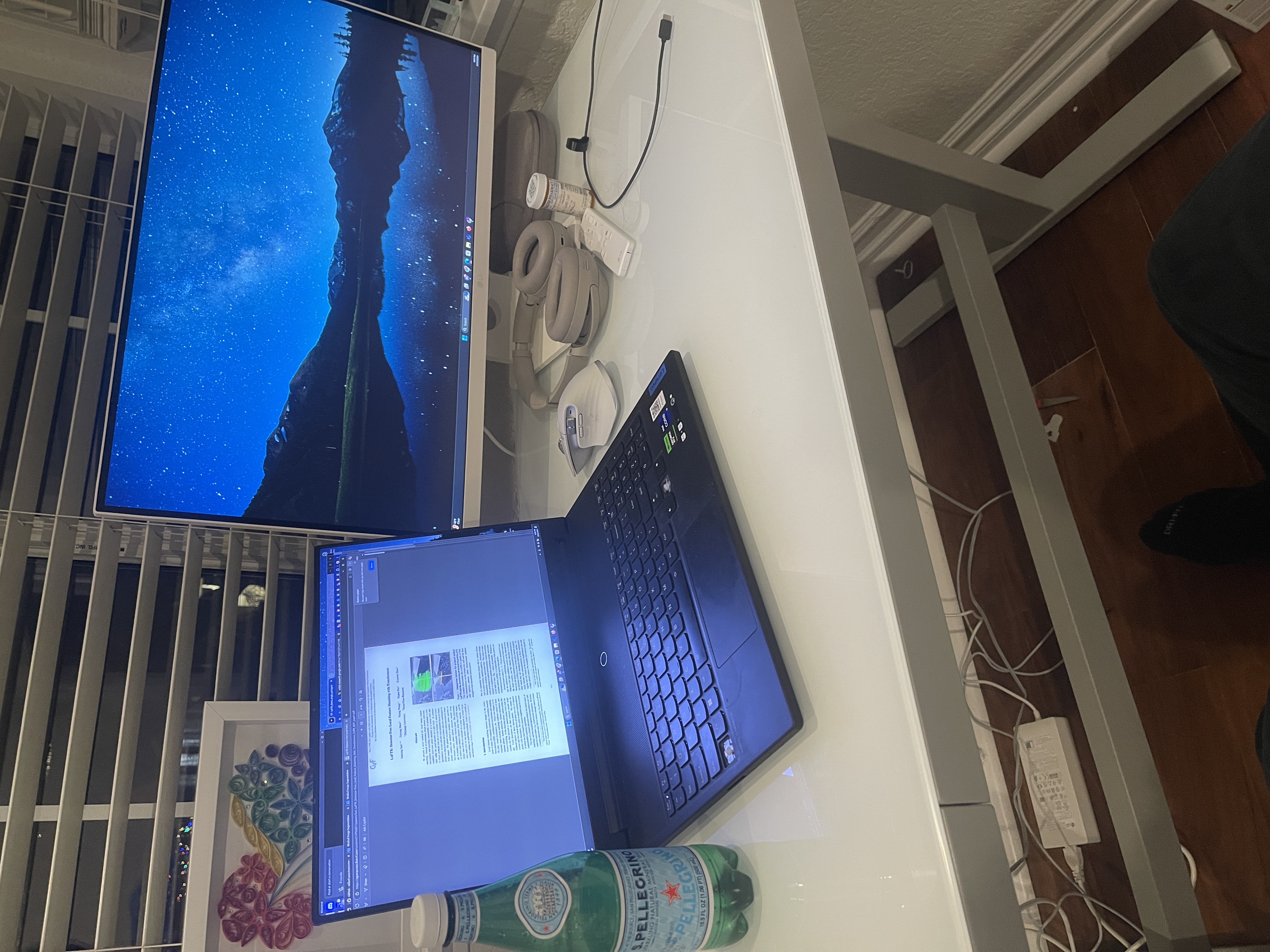
View 1 of the desktop setup

View 2 of the desktop setup

Here’s the code to run LoFTR on these images:

# Configure environment and download LoFTR code
!pip install torch einops yacs kornia
!git clone https://github.com/zju3dv/LoFTR --depth 1

# Load and preprocess images
img0_raw = cv2.imread(image_pair[0], cv2.IMREAD_GRAYSCALE)
img1_raw = cv2.imread(image_pair[1], cv2.IMREAD_GRAYSCALE)
img0_raw = cv2.resize(img0_raw, (640, 480))
img1_raw = cv2.resize(img1_raw, (640, 480))

img0 = torch.from_numpy(img0_raw)[None][None].cuda() / 255.
img1 = torch.from_numpy(img1_raw)[None][None].cuda() / 255.
batch = {'image0': img0, 'image1': img1}

# Inference with LoFTR
with torch.no_grad():
    matcher(batch)
    mkpts0 = batch['mkpts0_f'].cpu().numpy()
    mkpts1 = batch['mkpts1_f'].cpu().numpy()
    mconf = batch['mconf'].cpu().numpy()

When we ran this code on a pair of desktop setup images taken from slightly different angles, LoFTR was able to find 874 matching points between the images, demonstrating its robustness to viewpoint changes:

LoFTR Matches

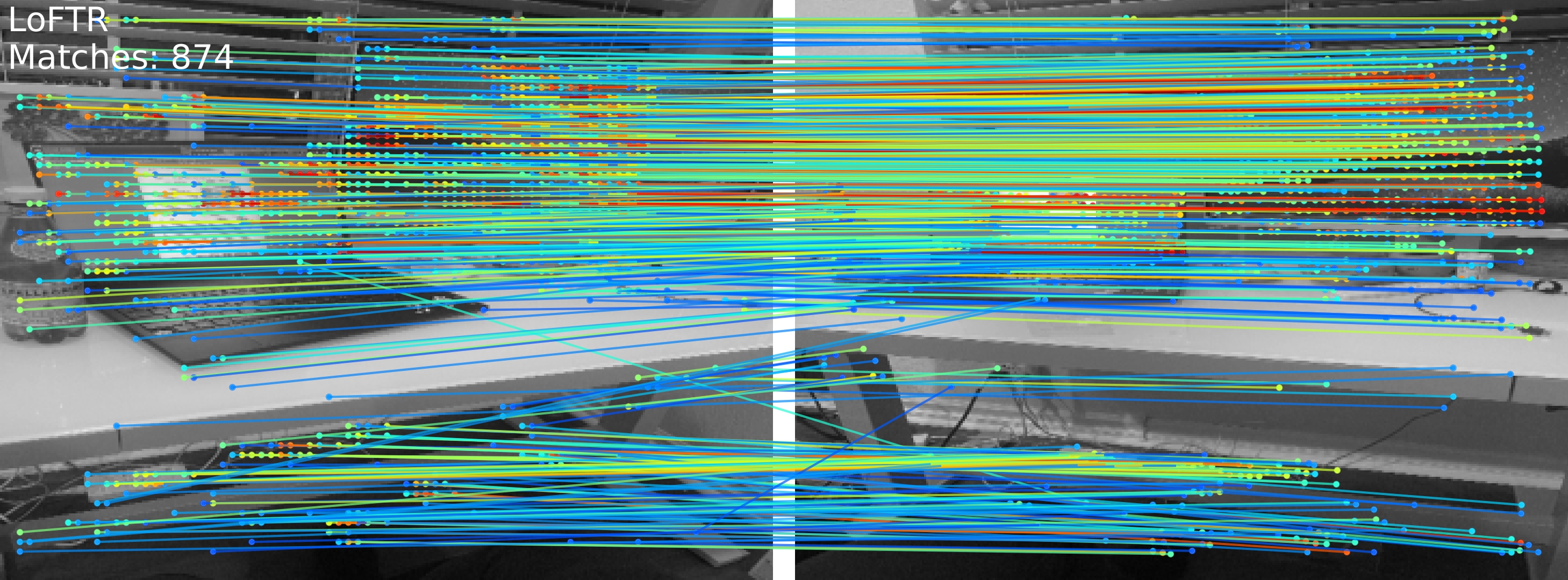
LoFTR matching points between two images of a desktop setup, showing 874 matches across various features including the laptop, monitor, and desk surface.

The colored lines indicate matched points between the two images, with different colors representing the confidence levels of the matches. As we can see, LoFTR successfully identified corresponding points across various features in the scene, including:

The laptop screen and keyboard
The external monitor displaying a mountain scene
The desk surface and its reflections
The window blinds in the background

This demonstrates LoFTR’s ability to handle:

Different viewing angles
Varied lighting conditions
Reflective surfaces
Complex indoor environments with multiple objects

3: Learning Super-Features for Image Retrieval

Motivation

Traditional feature detection and matching methods, such as using Convolutional Neural Network (CNN) features, have significant limitations. Methods like the Scale-Invariant Feature Transform (SIFT) detect keypoints individually and compute descriptors around these separate, independent keypoints. This approach ignores the spatial relationships between keypoints, making the method:

Sensitive to viewpoint changes.
Sensitive to lighting variations.

Even modern deep learning methods, such as CNN-based approaches, fail to consider spatial relationships. However, clusters of keypoints often contain rich contextual information. For example, a cluster of keypoints around a building edge has a predictable structure that can be recognized.

Techniques

To address these challenges and capture Super-Features, the paper introduces an iterative Local Feature Integration Transformer:

This method adapts pre-existing attention modules for image retrieval tasks.
During training, the loss is directly applied to Super-Features, and no additional labels or annotations are required beyond the image data itself.

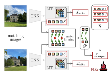
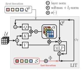
Figure x: The training process for the Local Feature Integration Transformer (FIT)
(image source: [3])

Architecture

The proposed framework follows a multi-step process to generate Super-Features:

Feature Extraction Backbone:
- A backbone CNN extracts dense feature maps that encode local patterns and textures from the input image.
Super-Feature Extraction:
- The framework detects salient regions from the feature maps. These regions capture spatial and geometric context that is meaningful for retrieval.
Context-Aware Processing:
- The framework uses non-local attention mechanisms to incorporate spatial relationships across the image.
- These attention modules allow the model to focus on non-adjacent regions in the image, ensuring that features capture long-range dependencies.
Training Objective:
The network minimizes losses for both:
- Keypoint Detection: Ensures that detected keypoints are repeatable across transformed images.
  - Loss Function: Cross-Entropy Loss.
- Descriptor Matching: Ensures that corresponding keypoints in two images have similar descriptors.
  - Loss Function: Triplet Loss.

How It Works

Input: A reference image from the dataset and a query image are fed into the network.
Feature Map Generation: Dense feature maps are extracted using the backbone CNN.
Keypoint and Descriptor Extraction:
- The framework detects keypoints and computes context-aware descriptors from the feature maps.
Matching: These context-rich features enable better comparison between images, resulting in more accurate image retrieval.

Results

The paper evaluates the proposed method, FIRe (Feature Integration-based Retrieval), against state-of-the-art techniques. The network is trained on the SfM-120k dataset. Key results include:

Memory Efficiency:
- Other methods required a minimum of 7.9 GB for the full R1M image set.
- The FIRe method used only 6.4 GB.
Accuracy Improvements:
- On the R-Oxford + R-1M hard sets, FIRe achieved an improvement of 3.3 points.
- On the R-Paris + R-1M hard sets, the improvement was as high as 12.2 points.
  - R-Oxford and R-Paris are datasets containing buildings from Oxford, England and Paris, France, respectively.
  - R-1M is a distractor dataset that aims to emulate real image retrieval tasks by adding irrelevant images that do not belong to the same categories as the other datasets

These results demonstrate that FIRe outperforms existing methods both in terms of accuracy and memory efficiency.

4: Improving Approximate Nearest Neighbor Search through Learned Adaptive Early Termination

Motivation

Efficient approximate nearest neighbor (ANN) search is essential for many applications, such as:

Image search
Recommendation systems
Sequence matching

ANN search aims to balance efficiency and accuracy, but it often relies on fixed configurations applied to all queries, which can lead to computational inefficiencies. Some queries require significantly more effort to find the nearest neighbor, making the process inefficient.

In this study, the researchers propose a learned adaptive early termination method. This method:

Predicts the optimal stopping point for each query.
Reduces latency without compromising accuracy.

Technique/Architecture

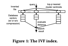
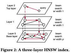
The architecture includes a Gradient Boosting Decision Tree (GBDT)-based regression model, using the LightGBM library, that outputs the predicted termination threshold for each query for three different indexes approaches (IVF, HNSW, IMI) with static and runtime features both combined as input to the model. This essentially learns and predicts when to stop searching for a certain query.

Latency Results (image source: [4])

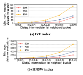
Distance between the query and its intermediate first neighbor for each index (image source: [4])

Results

The proposed adaptive method outperformed static configurations in terms of latency at the same recall levels for both the inverted file index (IVF) and hierarchical navigable small world graphs (HNSW) indices.

For applications targeting 95-100% recall-at-1 accuracy, without using vector compression, the method significantly reduced end-to-end latency across three million-scale datasets (DEEP10M, SIFT10M, GIST1M).

Key findings include:

VF index: Achieved up to a 58% reduction in latency (equivalent to a 2.4x speedup).
HNSW index: Achieved up to 86% reduction in latency (equivalent to a 7.1x speedup).

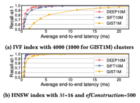
End-to-end latency results (image source: [4])

Latency Results (image source: [4])

Beyond Images: Feature Extraction in Genomics

While we’ve focused on image retrieval, the concepts of feature extraction and similarity search can be applied to many other domains. Here, we demonstrate an interesting application in genomics using the same fundamental principles. You can find our implementation in Google Colab.

Just as CNNs can extract meaningful features from images, we can use specialized models like DNABERT-2 to extract features from DNA sequences. Here’s our implementation of a DNA sequence similarity search:

def mystery_function(read):
    # Convert DNA sequence to numerical representation
    inputs = tokenizer([read], return_tensors='pt', padding=True)["input_ids"]
    
    # Get sequence embeddings from DNABERT-2
    hidden_states = model(inputs)[0]
    
    # Create a single vector representation via mean pooling
    read_representation = torch.mean(hidden_states, dim=1)
    
    # Calculate similarity with database sequences
    similarities = cosine_similarity(read_representation.detach().numpy(), 
                                  embedding_mean.detach().numpy())
    
    # Find and return top 5 most similar sequences
    top_indices = similarities.argsort()[0][-5:][::-1]
    for index in top_indices:
        print(dna_sequence_list[index], "similarity score:", similarities[0][index])

When we query this system with a DNA sequence ‘ACAGCTCTCCCC’, we get results like:

CGGCTAGGGATCGAACTCCGCGCGAGTGCC similarity score: 0.9912246
TCTGTGTTTGTTGAGTCTCCTGAGACTCCC similarity score: 0.98853076
TTAAACAGGTGGGTTCTATAGGTCTTACAT similarity score: 0.9881238
TGCCCCGGTGTAGAACGATCCGTGCACGCG similarity score: 0.98796815
CAGGTTAGACGGAGGTGCCGGTTTCCAGGG similarity score: 0.98769104

This demonstrates several interesting parallels with image retrieval:

Feature Extraction: Just as CNNs extract features from images, DNABERT-2 extracts features from DNA sequences by converting them into high-dimensional vectors (embeddings).
Similarity Metrics: We use cosine similarity to compare DNA sequence embeddings, similar to how we compare image feature vectors in CBIR systems.
Nearest Neighbor Search: The system returns the most similar sequences from a database, analogous to how image retrieval systems return visually similar images.

The high similarity scores (all above 0.97) suggest that our model captures meaningful patterns in the DNA sequences, allowing us to find similar genetic patterns just as we find similar visual patterns in images.

Reference

[1] Khuwaileh, M. “Extract a feature vector for any image with PyTorch.” Becoming Human: Artificial Intelligence Magazine. 2019.

[2] Sun, Jiaming, et al. “LoFTR: Detector-Free Local Feature Matching With Transformers.” Proceedings of the IEEE/CVF Conference on Computer Vision and Pattern Recognition (CVPR), 2021.

[3] Weinzaepfel, Philippe, et al. “Learning super-features for image retrieval.” Proceedings of the International Conference on Learning Representations (ICLR). 2022.

[4] Li, Conglong, et al. “Big Learning: A Study of Multi-Task Learning Algorithms for Large-Scale Data.” Carnegie Mellon University, Parallel Data Laboratory. 2016.