Novel View Synthesis with 3D Gaussian Splatting
Gaussian Splatting is a novel 3D reconstruction algorithm, radically improving the generation time compared to NeRFs using 3D Gaussians. In this project, we review its implementation as well as several applications of the more capable 3D reconstruction algorithm.
- Problem Statement
- Background
- 3D Gaussian Splatting
- Applications
- Running Existing Codebases
- References
Problem Statement
Our problem statement is the following: given a set of sparse images, how can we construct a corresponding 3D scene? [1]
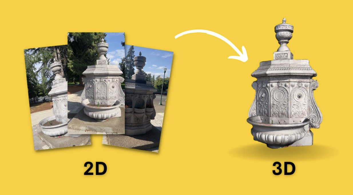
Fig 1. Problem Statement image [1].
Background
Structure From Motion
Structure from Motion (SfM) was an early solution to this problem. It transforms inputs of 2D images to a sparse point cloud. It does this through 2D image alignment, in which distinctive features are matched in each image, the camera pose is estimated, and the 3D coordinates are calculated. COLMAP is a package and CLI that implements SfM, allowing a user to easily generate the sparse point clouds through SfM.
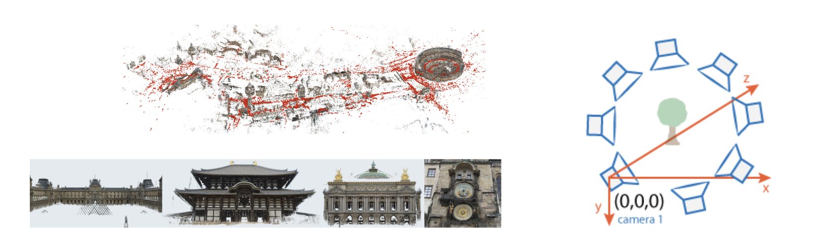
Fig 2. SfM
Neural Radiance Fields (NeRFs)
Similarly to SfM, given set of 2D images + camera poses, NeRFs also generates 3D scene. However, it revolutionized 3D reconstruction by representing 3D scenes with neural networks rather than mesh-based representations. This allows us to represent fine scene geometry, using a raycasting algorithm. In addition, since it’s implicitly represented, only requiring the MLP weights, the storage costs are small. However, this implicit representation makes rendering times large. In addition, downstream tasks such as scene editing and mesh generation are more difficult.
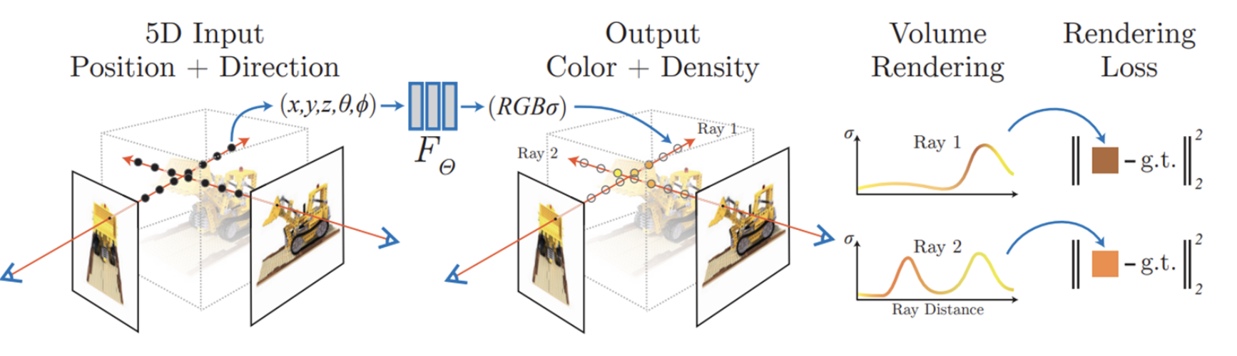
Fig 3. NeRFs
3D Gaussian Splatting
3D Gaussian Splatting consists of a three-step process
- Scene representation with 3D Gaussians
- 3D Gaussian optimization
- Real-time rendering algorithm
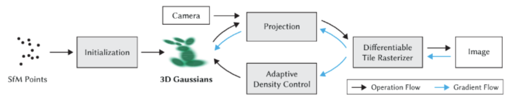
Fig 4. Gaussian Splatting Pipeline.
3D Gaussians
3D Gaussians are initialized by a set of 3D points from SfM and characterized by 4 parameters:
- Mean 𝜇 (3D point)
- Covariance matrix Σ
- Opacity 𝛼
- Color c (spherical harmonics coefficients)
Fig 5. Effect of Gaussian parameters on a 3D Gaussian point.
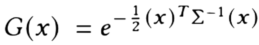
Fig 6. Gaussian Splatting Equation.
3D Gaussian Optimization
Gaussian optimization is the optimization process that gradually refines the rendering of the 3D scene through Iterations of rendering and comparison with training views. Fine-grained Adaptive control of Gaussians can be achieved by focusing on regions with missing geometric features and regions where Gaussians cover large regions. To do this, two basic operations are performed:
- Small Gaussians in under-reconstructed regions are cloned
- Large Gaussians in regions of high variance split up into two new Gaussians
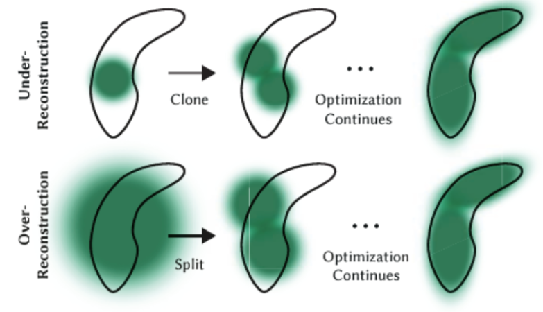
Fig 7. Algorithm for under/over-reconstructed regions during Gaussian optimization..
Comparisons with the rendered and training images use a combination of L1 Loss and D-SSIM Loss, defined as (𝜆 is a hyperparameter; it is set to 0.2 in the original paper):
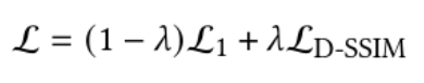
Fig 8. 3D GS Loss.
3D Gaussian Rasterizer
Finally, the 3D Gaussian Rasterizer is what is responsible for actually rendering the Gaussians in the 3D scene. As opposed to traditional geometric primitives/shapes like triangles and polygons, the 3D Gaussian Rasterizer renders Gaussian blots. To create a rendered view, the rasterizer projects 3D Gaussian distributions into a 2D image plane using a perspective or orthogonal projection, mimicking how a camera sees a 2D plane. To achieve blending and accumulation, the Rasterizer blends overlapping Gaussians by accumulating their contributions to pixel values in the rendered image using alpha blending or similar techniques to simulate transparency and lighting effects. To achieve depth ordering and occlusion handling, the Rasterizer makes it so that closer Gaussians occlude farther ones which might involve sorting Gaussians or using depth-buffer-mechanisms. Finally, to achieve light and shading effects, the Rasterizer incorporates shading effects by adjusting intensity and color of Gaussians based on lightning conditions.
Results
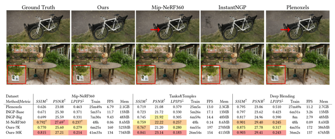
Fig 9. 3DGS Results.
Applications
3D Gaussian splatting can be used for many different applications. We will cover a few here:
Geometry Editing
Definition:
Geometry editing refers to modifying the spatial arrangement, structure, or properties of 3D blobs to define the underlying surface shape or characteristics of a 3D object
Examples:
Rigid Transformations: Moving, rotating, or scaling the object or parts of it. Non-Rigid Deformations: Stretching, bending, or warping parts of the object for more complex shape changes. Topology Adjustments: Adding or removing Gaussians to represent changes in the model’s topology (e.g., splitting a face or creating holes).
Advancements:
Utilizing surface priors and explicit deformation methods to optimize Gaussian parameters and number Frosting Layer
Techniques:
Mesh-Based Editing: Combining Gaussian Splatting with conventional meshes to use mesh vertices for parameterizing Gaussian positions. This enables real-time edits but is limited in flexibility for significant topology changes. Regularization and Surface Priors: Using priors like surface normals and gradients from explicit deformation methods to maintain consistency during edits. Topology Optimization: Advanced methods like face splitting or adding Gaussians to dynamically adjust the model’s topology.
Challenges:
Large-Scale Deformations: Significant changes in shape can be difficult because the relationship between Gaussians and the object surface might become inconsistent. Topology Modifications: Traditional GS struggles with modifying the connectivity or structure of the object, as Gaussians are often tied to a fixed mesh or surface.
Appearance Editing
Definition:
Focuses on visual attributes of 3D objects, such as their color, texture, shading, and material properties rather than geometric properties. Gaussians in GS can store additional attributes like color, opacity, and texture information.
Examples:
Texture Painting: Adding or altering textures on the object’s surface. Material Editing: Changing reflectivity, transparency, or other material properties. Lighting and Shadows: Adjusting how light affects the object, enabling relighting. Object Inpainting: Filling in missing or occluded regions to restore or create new details.
Techniques:
Language-Guided Editing: Using diffusion models (e.g., GaussianEditor) with natural language input to make targeted changes in appearance. Disentanglement: Separating geometry from appearance to allow independent modifications of texture and lighting (e.g., TextureGS and 3DGM). Mask-Based Updates: Applying segmentation models to isolate regions for editing while preserving surrounding details. Depth and Cross-Attention: Techniques like GaussCtrl and Wang et al. use depth maps or multi-view cross-attention to ensure consistency across perspectives.
Challenges:
Consistency: Ensuring that changes to appearance align with the object’s geometry across different views. Interdependence: Appearance attributes like texture and lighting are intertwined with geometry, making disentanglement and independent editing complex. Complexity: High-quality edits require accounting for multi-view consistency and realistic rendering constraints.
Physical Simulation
Definition:
Supports realistic simulations for fluid dynamics, motion, and collisions. Physical properties like mass, velocity, and surface normals are encoded into Gaussian parameters for simulation purposes.
Applications:
Solid and Fluid Dynamics: Simulating interactions between solids (e.g., deformable objects) and fluids (e.g., water, smoke). Physically-Based Rendering: Incorporating realistic reflections, refractions, and lighting effects based on physical interactions. Dynamic Behavior: Modeling real-world behaviors like elasticity, collisions, and deformation using particle-based dynamics.
Techniques:
Particle-Based Dynamics (PBD): Gaussian Splashing integrates 3DGS with PBD to simulate cohesive dynamics, including solid-fluid interactions and dynamic rendering. Continuum Deformation: PhysGaussian applies deformation models to Gaussian kernels, simulating physically realistic changes in shape and rendering. Spring-Mass Models: Spring-Gaus employs spring-mass systems to simulate dynamic properties, extracting parameters like mass and velocity from real-world inputs like videos. Surface Alignment: Normal-based alignment ensures that Gaussians conform to realistic surface orientations, improving physical and visual consistency.
Challenges:
Realism: Achieving physically accurate results while maintaining computational efficiency. Integration: Combining simulation with rendering and other Gaussian attributes like appearance or geometry. Dynamic Adaptation: Adjusting Gaussian parameters dynamically to reflect changing physical states (e.g., deformation, splitting).
Mesh Extraction (SuGaR)
The goal of SuGaR is to produce a method to quickly and efficiently extract meshes from 3D Gaussian Splatting. SuGaR introduces the following methods to assist in mesh extraction: regularization, mesh extraction through poisson reconstruction, and an optimizer.
In vanilla 3DGS, the Gaussians do not generally have an ordered structure or correspond well to the scene’s surfaces. This makes it extremely difficult to extract meshes from the Gaussians. To combat this, a regularization term is added into the Gaussian Splatting optimization that helps align the Gaussians with the scene surface while also being evenly distributed over the surface. This is done through deriving a Signed Distance Function assuming that the Gaussians already have the desired properties, and then minimizing the differences between this SDF and the actual one computed by the Gaussians. The regularization term is defined as:
\[\mathcal{R} = \frac{1}{|\mathcal{P}|} \sum_{p \in \mathcal{P}} |\hat{f}(p) - f(p)|\]where \(f(p) = \pm s_{g*} \sqrt{- 2 \log(d(p))}\), the “ideal” distance function associated with the density function $d$, $\hat{f}(p)$ is the estimate of the SDF of the surface currently created by the Gaussians, and $\mathcal{P}$ is the set of sampled points.
Another regularization term is also added to encourage the normals of SDFs \(f\) and \(\hat{f}\) to be similar:
\[\mathcal{R}_{\text{Norm}} = \frac{1}{|\mathcal{P}|} \sum_{p \in \mathcal{P}} \left\| \frac{\nabla f(p)}{\|\nabla f(p)\|_2} - n g^* \right\|^2_2\]For mesh extraction, Poisson reconstruction is run on sampled 3D points from a level set of the density computed from the Gaussians. To identify points on the level set with level parameter λ, points are first randomly sampled from the depth maps of the Gaussians as seen from the training viewpoints. For each randomly selected point, the line of sight is then sampled within 3 standard deviations of the 3D Gaussian in the direction of the camera to find a point on the level set. From these points, density values can then be calculated, and level set points and their normals can be found. Poisson reconstruction is then run on these points to construct a mesh.
How SuGaR samples points on the depth map for Poisson reconstruction:
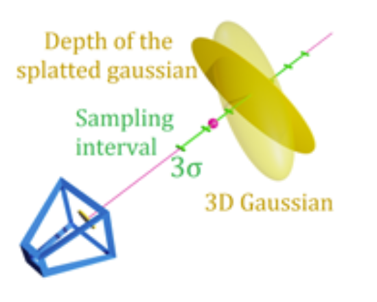
Fig 10. How SuGaR samples points on the depth map for Poisson reconstruction.
The mesh can then be further refined by initializing new 3D Gaussians on the mesh and using the Gaussian Splatting rasterizer to optimize. SuGaR outperforms many of the state-of-the-art methods for Novel View Synthesis using mesh and also outperforms some of the SOTA models that focus only on rendering. SuGaR also often has performance similar to SOTA models for rendering quality.
Deformable 3DGS
As mentioned, NeRFs struggle due to their slow speed, which makes it inefficient and ineffective. It’s constrained by ray-casting. This makes it impractical to generate dynamic scenes, where the objects are moving. However, 3DGS, by itself, also cannot effectively generate dynamic scenes. Inherently, it doesn’t understand the spatiotemporality of motion. This is shown by simply introducing a time-conditioned learnable parameter to 3DGS. Therefore, to make it compatible with dynamic scenes, we introduce a deformation field, which is essentially an MLP network mapping from each coordinate of 3D Gaussians and time to position, rotation, and scaling. Which we jointly learn this with the 3D Gaussians. This decouples motion and geometry structure, which introduces the geometric priors of the scene, associating changes in 3D Gaussians with both time and coordinates. The pipeline is as follows:
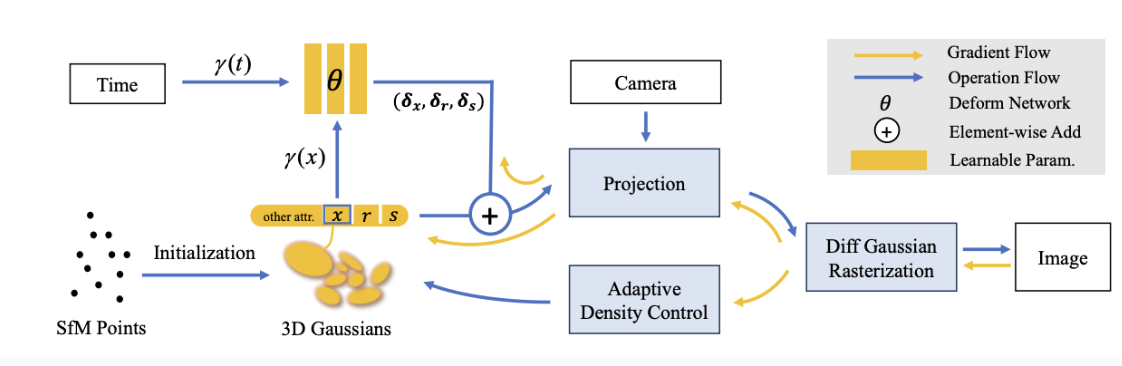
Fig 11. Deformable 3DGS pipeline
- From the SfM point clouds, we create our 3D Gaussians \(G(x, r, s, \sigma)\) (center position \(x\), opacity \(\sigma\), 3D covariance matrix from quaternion \(r\) and scaling \(s\). Spherical harmonics model the view-dependent appearance of each 3D Gaussian (viewing angle, changing light etc)
- We decouple the 3D Gaussians and the deformation field to model the 3D Gaussians that change over time. The deformation field takes in the positions of the 3D Gaussians with time \(t\), and outputs \(\delta x\), \(\delta r\), \(\delta s\)
- The deformed 3D Gaussians (\(G(x + \delta x, r+\delta r, s + \delta s, \sigma)\)) is rasterized using differential Gaussian Rasterization Pipeline, a tile-based rasterizer that allows \(\alpha\)-blending of anisotropic splats). The tile based approach ensures only tiles overlapping Gaussian’s footprint are rendered. In addition, the \(\alpha\)-blending combines multiple overlapping layers to create smooth, translucent effects. It determines pixel colors by blending Gaussian’s contribution with background based on opacity — this avoids sharp edges between overlapping Gaussians
- 3D Gaussians and deformation network can then be optimized jointly through fast backward pass.
DreamGaussian
DreamGaussian is a 3D content generation framework that adapts 3D Gaussian splatting for image-to-3D mesh generation. Previous iterations of 3D content generation frameworks utilized Neural Radiance Fields (NeRFs), but these approaches typically require hour-long optimizations that limit their use for real-world applications. DreamGaussian is inspired by the contributions of 3D Gaussian Splatting and Zero-1-to-3, a NeRF-based diffusion framework that synthesizes novel views of an object given a single input view [5].
DreamGaussian leverages the efficiency of 3D Gaussian Splatting by representing the 3D scene as a collection of small, localized Gaussian functions. 3D Gaussians are initialized randomly and then iteratively optimized to reconstruct the input, refining position, scale, and orientation of each Gaussian. A Score Distillation Sampling (SDS) loss distills 3D geometry and appearance from 2D diffusion models [6], minimizing the difference between the rendered images and the text prompt or, in our case, input images. SDS loss is defined as:
\[\nabla_\Theta \mathcal{L}_{SDS} = \mathbb{E}_{t,p,\epsilon}[w(t)(\epsilon_\phi(I^p_{RGB};t,\tilde{I}^r_{RGB},\Delta p) - \epsilon) \frac{\partial I^p_{RGB}}{\partial\Theta}]\]An overview of the DreamGaussian pipeline is as follows:
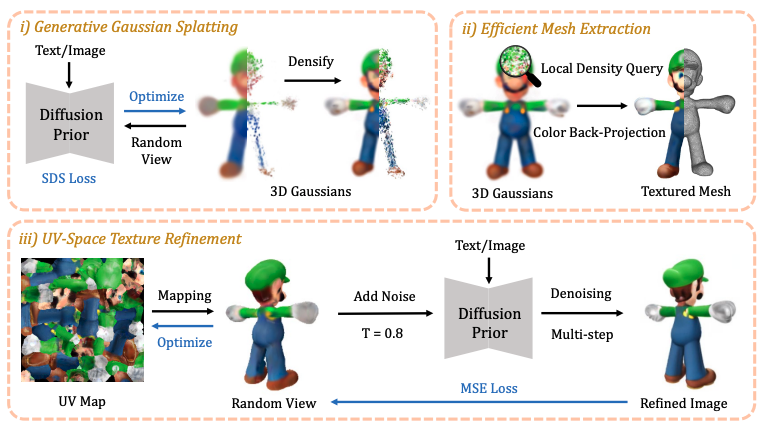
Fig 12. DreamGaussian framework for generation and mesh extraction
- Score Distillation Sampling is used to sample from the Zero-1-to-3 XL diffusion prior and densify the Gaussians
- A local density query algorithm is performed to extract mesh geometry. The Marching Cubes algorithm is adapted with culled Gaussians to reduce queries in blocks for efficient rasterization, and the weighted opacity of each 3D Gaussian is summed.
- The rendered RGB image is back-projected to the mesh surface and baked as the texture by unwrapping the mesh’s UV coordinates and sampling 9 azimuths and 3 elevations to render. This texture image serves as an initialization for texture fine-tuning.
- UV-Space texture refinement is performed to extract coarse texture from the mesh. A blurry image \(I^p_{coarse}\) is rendered from an arbitrary camera view \(p\), which is perturbed with a random noise and a multi-step denoising process \(f_\phi(\cdot)\) is applied using a 2D diffusion prior to obtain a refined image. A pixel-wise MSE loss is used to optimize the texture against the coarse image: \(\mathcal{L}_{MSE} = \|I^p_{fine} - I^p_{coarse}\|^2_2\).

Fig 13. Comparison of generation speed and mesh quality between DreamGaussian and previous works
DreamGaussian generates meshes of significantly higher quality compared to previous approaches, as illustrated in the views above.
Instant Splat
Task The goal of InstantSplat is to address the shortcomings of COLMAP when its randomly initialized Gaussians or sparse SfM points fail with sparse-view data or data with too few images and lacks an error correction mechanism which causes errors to build up over time. 3 Main Contributions: The overall architecture of Instant splat consists of a pipeline that integrates Multi-View Stereo (MVS) with 3D-GS to address sparse-view reconstruction in the reliance on SfM and training efficiency.
InstantSplat also introduces an efficient, confidence-aware point downsampler address scene overparameterization.
Finally, InstantSplat proposes a self-correction mechanism in the form of a gradient-based joint optimization framework using photometric loss to align the Gaussians and camera parameters in a self-supervised manner.

Fig 14. InstantSplat Framework
Running Existing Codebases
Vanilla 3D Gaussian Splatting
We first ran vanilla 3D Gaussian Splatting as described in the foundation paper to reconstruct scenes. We obtained the following results with the provided example images:

Fig 15. Vanilla 3D Gaussian Splatting train scene

Fig 16. Vanilla 3D Gaussian Splatting truck scene
There are noticeable artifacts present in the final splats, as well as low-resolution surfaces with rough edges due to a shorter training time (~1 hour). Generated scenes would be of higher quality if trained for 48 hours as in the original 3DGS implementation, or by using an optimized method like InstantSplat. We attempted to run the scenes with the online InstantSplat demo, but it seems to not be currently maintained.
DreamGaussian
We ran DreamGaussian on a single view of a T-Rex from the D-NeRF synthetic dataset, which was used to benchmark Deformable 3D Gaussian Splatting. We obtained the following result, placed alongside the Deformable 3DGS render for comparison. For context, the original scene contains 220 training views for training and validation.
Fig 17. Render of T-Rex with Deformable 3DGS

Fig 18. Render of T-Rex with DreamGaussian (single input view)
Multi-view Gaussian splatting methods still significantly outperform single-view methods in terms of reconstruction quality. However, these generative methods can serve as a solid baseline for efficient 3D content creation, especially given that it requires just a single view and the model outputs a solid mesh that can be easily modified. Single-view applications of 3D Gaussian Splatting are still a very active area of research.
References
[1] Kerbl, Bernhard, Kopanas, Georgios, Leimkühler, Thomas, and Drettakis, George. 3D Gaussian Splatting for Real-Time Radiance Field Rendering. ACM Transactions on Graphics, 42(4), July 2023.
[2] Yang, Ziyi, et al. “Deformable 3d Gaussians for high-fidelity monocular dynamic scene reconstruction.” Proceedings of the IEEE/CVF Conference on Computer Vision and Pattern Recognition. 2024.
[3] Tang, Jiaxiang, Ren, Jiawei, Zhou, Hang, Liu, Ziwei, and Zeng, Gang. DreamGaussian: Generative Gaussian Splatting for Efficient 3D Content Creation. arXiv preprint arXiv:2309.16653, 2023.
[4] Guédon, Antoine, and Vincent Lepetit. “Sugar: Surface-aligned Gaussian splatting for efficient 3d mesh reconstruction and high-quality mesh rendering.” Proceedings of the IEEE/CVF Conference on Computer Vision and Pattern Recognition. 2024.
[5] Liu, Ruoshi, et al. Zero-1-to-3: Zero-Shot One Image to 3D Object. arXiv:2303.11328, arXiv, 20 Mar. 2023. arXiv.org, https://doi.org/10.48550/arXiv.2303.11328.
[6] Poole, Ben, et al. DreamFusion: Text-to-3D Using 2D Diffusion. arXiv:2209.14988, arXiv, 29 Sept. 2022. arXiv.org, https://doi.org/10.48550/arXiv.2209.14988.
[7] Fan, Zhiwen, Cong, Wenyan, Wen, Kairun, Wang, Kevin, Zhang, Jian, Ding, Xinghao, Xu, Danfei, Ivanovic, Boris, Pavone, Marco, Pavlakos, Georgios, Wang, Zhangyang, and Wang, Yue. InstantSplat: Unbounded Sparse-view Pose-free Gaussian Splatting in 40 Seconds. arXiv preprint arXiv:2403.20309, 2024.