Anomaly Detection
Anomaly detection is a critical task in domains such as cybersecurity, healthcare, and fraud detection. It involves identifying patterns in data that deviate significantly from the norm. This report compares three state-of-the-art approaches to anomaly detection: a clustering-based method, a GAN-based method, and a reinforcement learning (RL)-based method. Each approach leverages unique architectures and methodologies to address the challenge of detecting anomalies in various datasets. This comparative analysis evaluates these models across key dimensions: datasets, architectures, and results.
- Introduction
- GANomaly: Semi-Supervised Anomaly Detection via Adversarial Training
- DPLAN Semi-Supervised Reinforcement Learning-Based Approach
- Clustering-Based Approach
- Conclusion
- References
Introduction
Anomaly detection is a critical task in domains such as cybersecurity, healthcare, and fraud detection. It involves identifying patterns in data that deviate significantly from the norm. This report compares three state-of-the-art approaches to anomaly detection: a clustering-based method, a GAN-based method, and a reinforcement learning (RL)-based method. Each approach leverages unique architectures and methodologies to address the challenge of detecting anomalies in various datasets. This comparative analysis evaluates these models across key dimensions: datasets, architectures, and results.
GANomaly: Semi-Supervised Anomaly Detection via Adversarial Training
The first approach to the unique problem of distinguishing unknown anomalies introduces a modified adversarial autoencoder with an encoder-decoder-encoder structure. Essentially, the model first learns to reconstruct normal images using a clean dataset of only non-anomalous images. Consequently, it should struggle to recreate anomalous images. The idea for this proposal was based off Schlegl et al.’s hypothesis that the latent vector learned by GANs represent the true distribution of the data, with the exception that optimizing the GAN would be very computationally expensive. One key difference between Ackay, Atapoou-Abarghouei, and Breckon’s approach and previous GAN and AE networks is that their approach does not require two-stage training and is efficient both during training and inference.
Taking a sneak peek into the structure of this network we see that the first encoder network maps the input images into a latent representation, which is then used to reconstruct a generated output. A second encoder then maps the generated image to another representation. The modified GAN network infers the distribution for non-anomalous images by minimizing the distance between generated images and their latent vectors. When running new, potentially anomalous, images through the network, it is expected that anomalous ones will have a larger distance from their learned distribution.
Network Architecture:
Training Dataset \(D\) consists of M normal images.
\[D = \{X_1, X_2, \dots, X_M\}\]Smaller Test dataset \(\widehat{D}\) of \(N\) normal and abnormal images.
\(\widehat{D} = \{(\widehat{X}_1, y_1), \dots, (\widehat{X}_N, y_N)\}\) where \(y_i \in [0, 1]\)
The generator subnetwork \(G\) consists of two components, \(G_E(x)\), the encoder, and \(G_D(z)\), the decoder.
\(G_E(x)\) uses a convolutional layer followed by batch-norm with a leaky \(ReLU()\) activation function and compresses the output into a vector, \(z\).
\(G_D(z)\) uses the same architecture as DCGAN which consists of convolutional transpose layers, \(ReLU()\) activation function, and batch norm finished by a tanh layer. This decoder essentially upscales \(z\), reconstructing the original input image \(x\) as \(\widehat{x}\).
The second subnetwork in GANomaly is \(E\) which compresses \(\widehat{x}\) and returns \(\widehat{z}\), a vector representation for the generated \(\widehat{x}\) with the same dimensions as the latent vector \(z\).
Lastly, the discriminator network, \(D\) is also the same as the discriminator network in DCGAN.
The hypothesis is founded in the idea that when an abnormal image is passed into \(G\), \(G_D\) will not be able to reconstruct the abnormalities from the latent vector \(z\). The second encoder would consequently map \(\widehat{x}\) to \(\widehat{z}\) with additional missed feature representations resulting in a greater difference between \(z\) and \(\widehat{z}\).
Objective Function
The objective function is a combined loss of three functions each optimizing one of the networks described above.
Adversarial Loss aims to minimize \(L_2\) distance between the feature representation of the original image and generated images. The formal definition for this loss is below.
\[L_{adv} = \mathbb{E}_{x \sim p_X} \| f(x) - \mathbb{E}_{x \sim p_X} f(G(x)) \|_2\]Contextual Loss minimized the difference between input images and generated images and in defined below.
\[L_{con} = \mathbb{E}_{x \sim p_X} \| x - G(x) \|_1\]An additional Encoder Loss is used to minimize the distance between \(z\), the bottleneck features of the input, and \(\widehat{z}\), the encoded features of the generated image.
\[L_{enc} = \mathbb{E}_{x \sim p_X} \| G_E(x) - E(G(x)) \|_2\]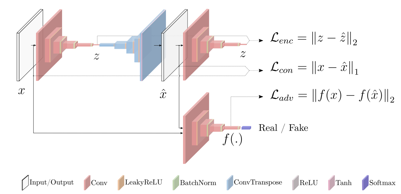
Fig. 1 Pipeline of GANomaly approach[2]
Testing
During test time, the encoder loss is used to score the abnormality, \(A(\widehat{x})\), of an image, and an abnormality over a certain threshold is used.
\[A(\widehat{x}) = \| G_E(\widehat{x}) - E(G(\widehat{x})) \|_1\]Scores from the entire test data are stored in a set \(S\) defined \(S = \{ s_i : A(\widehat{x}_i), \widehat{x}_i \in \widehat{D} \}\) which is then scaled by the formula below to return a vector, \(S'\), used to evaluate the model. \(s'_i = \frac{s_i - \min(S)}{\max(S) - \min(S)}\)
Experiment Setup & Results
GANomaly was tested and evaluated on 4 datasets. The first is the MNIST dataset in which each class was separated from training data and then used to represent the anomalous class. The second is the CIFAR10 dataset, which was evaluated the same way as MNIST, just with more complex images. The last two datasets, the University Baggage Anomaly (UBA) Dataset and Full Firearm vs. Operational Benign (FFOB) were used to evaluate the model in a practical setting. In each of the last two, abnormal classes are explicitly defined.
Based on the AUC of the ROC, GANomaly significantly outperforms previous research in both the MNIST and CIFAR10 dataset. For the UBA and FFOB datasets, this model again outperforms other models except in the knife anomaly category, which is comparable. The lower performance in this category is due to the fact that the simple shape of knives causes overfitting and results in a lot of false positives.
Several hyperparameters were also tuned in the testing process. It was discovered that the best choice for the size of the latent vectors \(z\) and \(\widehat{z}\) was 100 and the optimal weights for the 3 losses were \(w_{adv} = 1\), \(w_{con} = 50\), and \(w_{enc} = 1\) in the MNIST dataset. These hyperparameters were also used to train the rest of the models.
Additionally, the efficiency of this model achieves the best runtime compared to other models. Notably, the runtime performances for the UBA and FFOB datasets are comparable to MNIST despite their image and network size being more than twice the size.
DPLAN Semi-Supervised Reinforcement Learning-Based Approach
The next approach for anomaly detection attempts to use both labeled and unlabeled data. In anomaly detection a major problem is the lack of labeled anomaly data. Most labeled anomaly datasets are small and do not properly characterize the many different types of anomalies that exist. However, most applications where anomaly detection would be used has large scale unlabeled data that contain diverse anomalies not represented in a labeled dataset. To address the issues stemming from relying on only labeled or unlabeled data sets, Pang et. al proposes Deep Q-Learning with Partially Labeled ANomlaies (DPLAN). This is a semi-supervised reinforcement learning based-approach which leverages both labeled anomaly data to learn known anomalies while also exploring new anomalies in unlabeled data.
Model
Architecture Overview
DPLAN is based off of a reinforcement learning model which has four main components.
Action Space: Two possible actions - labeling a sample as either \(a^0\) (normal) or \(a^1\) (anomalous)
Environment: An anomaly Biased sampling function \(g(s_{t+1} \mid s_t, a_t)\) to supply the agent with states. These are two parts of this sampling function.
There is a uniform sampling function to sample a state which in this case is an observation from the labeled anomaly dataset \(D^a\)
\[g_a \sim U(D^a)\]There is also a function that samples from the unlabeled dataset. This function attempts to sample an observation that is most likely to be an anomaly. To do this, if the past observation resulted in an anomaly it samples the datapoint closest to it in the unlabeled space else if the past observation did not result in an anomaly it tries to grab the data point farthest from it in the unlabeled space.
\[g_u(s_{t+1} \mid s_t, a_t; \theta_e) = \begin{cases} \arg \min\limits_{s \in S} d(s_t, s; \theta^e) & \text{if } a_t = a^1 \\ \arg \max\limits_{s \in S} d(s_t, s; \theta^e) & \text{if } a_t = a^0 \end{cases}\]Between these two sampling techniques, \(g_a\) will occur with probability p of the time while \(g_u\) will occur with probability 1-p of the time. By default, p is 5%.
Agent: A Neural Network seeking the optimal action of either choosing \(a^0\) or \(a^1\). The agent in DPLAN is implemented using a deep Q-network (DQN).
In a DQN a Q-value or (quality value) for each state-action pair is computed to evaluate the potential reward of each action in a given state. The network learns the value of classifying a specific observation as either ‘normal’ or anomalous’ through an iterative learning process. In each iteration, the DQN takes an action, receives the reward for the action, and updates its Q-values to maximize the cumulative rewards over time.
Reward Function: Two reward functions are used, an external reward which rewards the agent for properly calling a labeled anomaly an anomaly, and a intrinsic reward function which rewards the agent for exploring novel data. The total reward is based on the combination of these two functions.
The external reward function encourages the agent to correctly classify labeled anomalies as anomalies. To do this, it increases rewards when the agent properly predicts a labeled anomalous observation as an anomaly while also penalizing incorrect labels.
\[r_t^e = h(s_t, a_t) = \begin{cases} 1 & \text{if } a_t = a^1 \text{ and } s_t \in D^a \\ 0 & \text{if } a_t = a^0 \text{ and } s_t \in D^u \\ -1 & \text{otherwise} \end{cases}\]The intrinsic reward function encourages the agent to explore and classify potentially anomalous observations. It does this using the unsupervised anomaly detector iForestis based on the unsupervised anomaly detector iForest which gives a higher reward for observations farther from other data points in the feature species.
\[r_t^i = f(s_t; \theta^e) = \text{iForest}(s_t; \theta^e)\]The total reward function combines the external and intrinsic rewards.
\[r_t = r_t^e + r_t^i\]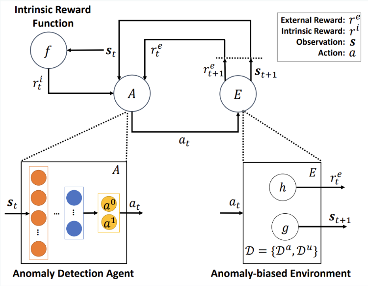
Fig. 2 DPLAN Framework[3]
Training
DPLAN follows a typical reinforcement learning training cycle.
- The agent receives an initial observation by the sampling function g from the environment
- Agent takes action \(a_t\) to maximize reward based on the current observation
- The next observation is obtained by the sampling function \(g(s_{t+1} \mid s_t, a_t)\) in the simulation environment where \(s_t\) is the current observation and \(a_t\) is the current action
- The reward function is used to update the agent based on the action
- Repeat the training process from step 2, using the next observation obtained
Results
The Area Under the Precision-Recall Curve (AUC-PR) and Area Under the Receiver Operating Curve (AUC-ROC) was evaluated across 13 datasets, comparing DPLAN with 5 competing methods, DevNet, Deep SAD, REPEN, iFOREST, and DUA. DPLAN performed the best out of these models on 10 of the 13 datasets.
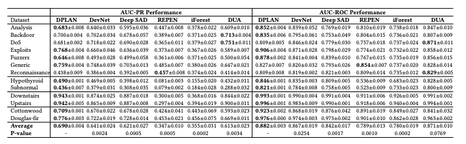
Table 1 AUC-PR and AUC-ROC Performance of DPLAN and five competing methods on 13 real-word datasets[3]
Clustering-Based Approach
Overview
Another approach to anomaly detection is clustering with deep learning and this is the method we chose to implement code for. This is talked about in the paper by Elie Aljalbout et al. it explains how deep learning enhances the ability to group data points based on their inherent similarity. By leveraging the representational power of neural networks, this approach integrates representation learning with clustering objectives to transform raw high-dimensional data into a clustering-friendly latent space.
Architecture
The proposed method employs a convolutional autoencoder, a neural network architecture designed for unsupervised representation learning. This structure consists of three main components:
- Encoder: Stacked convolutional layers extract hierarchical features from the input data, transforming it into a low-dimensional representation. The encoder outputs a latent vector ( z ) that represents essential information for clustering.
- Latent Space: The intermediate low-dimensional representation acts as the foundation for clustering. This space is optimized for separability and compactness.
- Decoder: Convolutional transpose layers reconstruct the original input from the latent representation. The decoder makes sure that critical information is preserved during encoding.
Autoencoder Training Loss
To train the autoencoder, a reconstruction loss is employed to minimize the difference between the input and its reconstruction. The reconstruction loss is expressed as:
\[L_{\text{AE}} = \frac{1}{N} \sum_{i=1}^N \| x_i - \hat{x}_i \|^2\]where ( x_i ) is the original input and (x̂ᵢ) is its reconstruction. This loss ensures that the latent space preserves information vital for clustering.
Loss Functions
To achieve effective clustering, the proposed approach combines two complementary loss functions:
1. Reconstruction Loss (\(L_{\text{AE}}\))
This loss ensures the latent space maintains important features of the original data, facilitating meaningful clustering. It has been defined above and encourages the encoder-decoder pair to accurately reconstruct the input data.
2. Clustering Loss (\(L_{\text{Cluster}}\))
The clustering loss optimizes the latent representation to form well-separated, compact clusters. Two specific implementations of clustering loss are:
a. k-Means Loss
This loss minimizes the distance between data points and their respective cluster centroids:
\[L_{\text{k-Means}} = \sum_{i=1}^N \sum_{j=1}^K r_{ij} \| z_i - \mu_j \|^2\]where:
- ( zᵢ) is the latent representation of the ( i )-th data point.
- ( μⱼ) is the centroid of cluster ( j ).
- ( rᵢⱼ) is a binary indicator denoting the assignment of ( zᵢ) to ( μⱼ).
b. Cluster Assignment Hardening Loss
This loss sharpens cluster assignments, making them more deterministic. It is based on the Kullback-Leibler (KL) divergence between the auxiliary distribution ( P ) and the predicted distribution ( Q ):
\[L_{\text{Cluster}} = KL(P \| Q)\]The auxiliary distribution ( P ) is defined as: \(p_{ij} = \frac{q_{ij}^2 / \sum_i q_{ij}}{\sum_{j'} \left( q_{ij'}^2 / \sum_i q_{ij'} \right)}\)
This formulation helps associate data points with a single cluster.
Combined Loss
The total loss function integrates reconstruction and clustering losses using a weighted combination:
\[L = \alpha L_{\text{Cluster}} + (1 - \alpha) L_{\text{AE}}\]Here, (α) is a hyperparameter that balances the trade-off between clustering performance and data reconstruction.
Training Procedure
The training process involves two distinct phases:
- Pretraining Phase:
- The autoencoder is optimized solely using the reconstruction loss (\(L_{\text{AE}}\)). This step initializes the latent space to represent the data accurately.
- Fine-tuning Phase:
- Both reconstruction and clustering losses are jointly optimized. The weight (α) is progressively increased to prioritize clustering while retaining essential reconstruction constraints.
Additionally, the method re-runs k-means clustering on the optimized latent space post-training to further refine cluster assignments.
Experimental Results
The proposed approach was evaluated on benchmark datasets like MNIST and COIL20. Key results include:
- MNIST: A dataset of 70,000 images of handwritten digits (28×28 pixels).
- COIL20: A dataset of 1,440 grayscale images of 20 objects (32×32 pixels).
Results show that taxonomy enables the creation of high-performing methods in a structured and analytical way. Researchers can selectively recombine or replace distinct aspects of existing methods instead of relying on experiment/discovery based approach.
Performance Metrics
The clustering performance was measured using:
- Clustering Accuracy (ACC): Fraction of correctly clustered data points.
- Normalized Mutual Information (NMI): Degree of correspondence between predicted and true cluster labels.
Results Summary
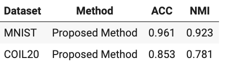
Table 2 Clustering Method Result[1]
Clustering Model Implementation
This clustering model did not have an existing code implementation. So we choose to create an implementation which follows the taxonomy and methodology outlines in the paper. The notebook we ran this on can be found here.
We choose to write an implementation and then use it to perform deep learning-based clustering on the MNIST dataset. Here’s an overview of the steps taken:
Library Setup and Data Loading: Necessary libraries are installed and imported. The MNIST dataset is loaded, combined (training and test sets), and preprocessed using transformations to convert images to normalized tensors.
Model Architecture:
-
Convolutional Autoencoder (CAE): Defined with an encoder compressing input images into a latent space and a decoder reconstructing images from this latent representation.
-
Clustering Layer: Implements a clustering mechanism that computes soft cluster assignments using the Student’s t-distribution based on the latent features.
-
Pre-training: The CAE is pre-trained using Mean Squared Error (MSE) loss to ensure that it learns meaningful feature representations by reconstructing input images accurately.
Clustering Initialization:
- K-Means Initialization: After pre-training, K-Means clustering is performed on the learned latent features to initialize cluster centers.
- Assignment of Cluster Centers: The initialized cluster centers from K-Means are assigned to the Clustering Layer to guide the clustering process.
Fine-tuning:
- The model is fine-tuned using a combined loss of reconstruction loss and clustering loss (KL Divergence). This joint training ensures that the latent space is optimized both for accurate image reconstruction and effective clustering.
- Target Distribution: A target distribution is computed to refine the cluster assignments, enhancing cluster compactness and separation.
Evaluation:
-
Clustering Performance Metrics: The model’s clustering performance is evaluated using Normalized Mutual Information (NMI) and Clustering Accuracy (ACC), showcasing its effectiveness compared to existing methods.
-
Visualization: t-SNE is employed to visualize the high-dimensional latent features in a 2D space, illustrating the separation and grouping of clusters relative to true labels.
Modularity and Best Practices:
- The implementation ensures modularity by separating the autoencoder and clustering components, facilitating maintenance and potential future enhancements.
Device-Agnostic Code:
- The code dynamically selects between GPU and CPU, ensuring compatibility across different execution environments.
Error Handling:
- Corrections were made to assign cluster centers to the appropriate layer, preventing attribute-related errors and ensuring smooth training.
The final results from running this model can be seen below.
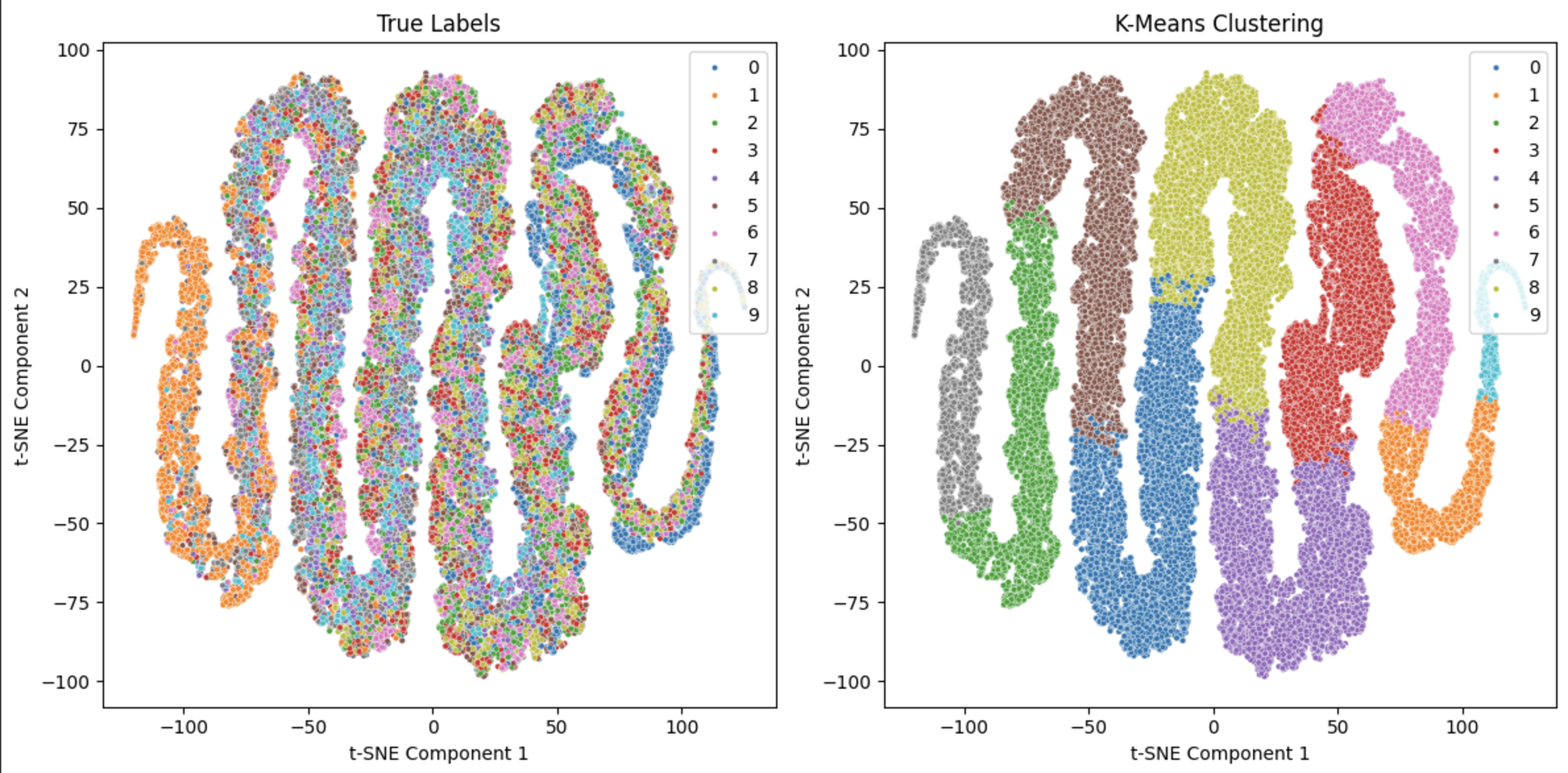
Fig. 3 Result of running code on MNIST
Conclusion
Anomaly detection remains a challenging problem for deep learning in the realm of computer vision and a critical application across many domains, from cybersecurity to healthcare. We examined and compared three novel approaches to anomaly detection: GANomaly, a GAN-based semi-supervised method; DPLAN, a reinforcement learning-based semi-supervised technique; and a clustering-based approach. Each method offers unique strengths tailored to specific datasets and challenges, as demonstrated by the results across various benchmarks. GANomaly excelled in reconstructing non-anomalous data and distinguishing anomalies by leveraging adversarial training, achieving superior performance on both synthetic datasets like MNIST and practical datasets such as UBA. DPLAN demonstrated the potential of reinforcement learning by leveraging both labeled and unlabeled data, addressing the challenges of anomaly diversity and dataset imbalance with an innovative reward-driven architecture. Lastly, the clustering-based approach provided a robust baseline, emphasizing simplicity and efficiency in scenarios with limited computational resources. The comparative analysis underscores that there is no one-size-fits-all solution in anomaly detection. Choosing the appropriate method depends largely on the application context, data available, and computational constraints.
References
-
Aljalbout, E., Golkov, V., Siddiqui, Y., Strobel, M., & Cremers, D. (2018). Clustering with deep learning: Taxonomy and new methods. arXiv preprint arXiv:1801.07648.
-
Akcay, S., Atapour-Abarghouei, A., & Breckon, T. P. (2018). GANomaly: Semi-supervised anomaly detection via adversarial training. arXiv preprint arXiv:1805.06725.
-
Pang, G., van den Hengel, A., Shen, C., & Cao, L. (2021). Toward deep supervised anomaly detection: Reinforcement learning from partially labeled anomaly data. In Proceedings of the 27th ACM SIGKDD Conference on Knowledge Discovery and Data Mining (pp. 1291–1300). ACM. https://doi.org/10.1145/3447548.3467417.
-
Radford, A., Metz, L., Chintala, S.: Unsupervised Representation Learning with Deep Convolutional Generative Adversarial Networks. In: ICLR (2016)