Visual Question Answering
(Open-answer) visual question answering (VQA** for short) is a computer vision task to: given an image and a natural-language question about the image, return an accurate and human-like natural-language response to the query using information in the image. Formally, the open-answer VQA task is: given an image-question pair
(I, q), output a sequence of characterss(of arbitrary length).
- Visual Question Answering
Visual Question Answering
Table of Contents
- Visual Question Answering
Introduction
(Open-answer) visual question answering (VQA for short) is a computer vision task to: given an image and a natural-language question about the image, return an accurate and human-like natural-language response to the query using information in the image. Formally, the open-answer VQA task is: given an image-question pair (I, q), output a sequence of characters s (of arbitrary length).
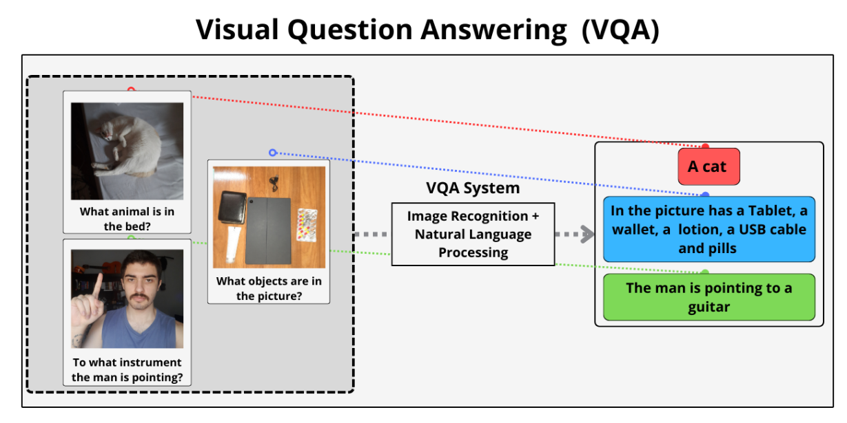
Fig 1: An illustration of the VQA task [3]
As a task, VQA is notable in that it extends existing vision/NLP tasks (e.g. image captioning, textual Q&A) by requiring multi-modal knowledge across two separate domains (image & natural language). Due to the open-endedness of VQA questions, a performant VQA model must have the capabilities to correctly answer a vast array of possible input queries across many different domains. This requires both a deep image understanding (as in image captioning) and a deep textual understanding (as in textual Q&A); however, it additionally requires the ability to combine knowledge across both domains to successfully answer questions. In this sense, VQA represents a “next step forward” in terms of building a compelling and challenging AI task.
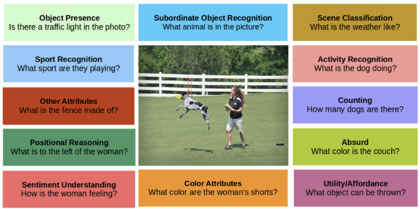
Fig 2: Aspects of the VQA task [9]
In particular, a key challenge in VQA is the requirement of common-sense reasoning. For example: to answer questions such as “Does this person have 20/20 vision?” and “Is this person expecting company” (pictured below), a VQA model must be able to both identify and extract the requisite information from relevant aspects of the image, reflecting a deeper notion of image understanding compared to previous image tasks.
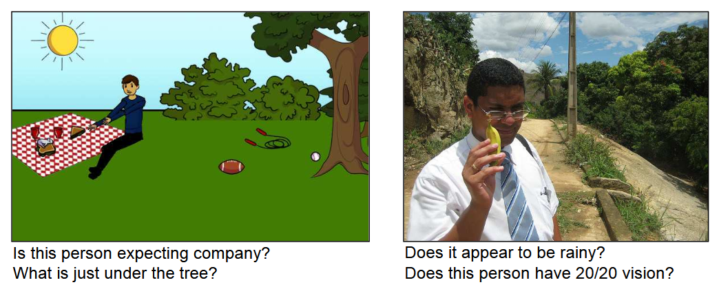
Fig 3: Reasoning tasks in VQA [2]
VQA
Most VQA architectures consist of two components – an encoder and a decoder – that perform the following sequence of steps:
- Encoder:
- Feature extraction: Extracts features from the image and natural-language inputs to compute text & image embeddings
- Multimodal fusion: Obtains a joint embedding from the image & text embeddings via a fusion method
- Decoder: Generates a natural-language response from the joint text & image embedding
In particular, most modern VQA models use a vision backbone (e.g. ResNet, ViT) and text encoder (e.g. Transformer) to compute separate image and text embeddings, then concatenate them to form a joint embedding. This joint embedding is then passed to a large language model/LLM to output the final vector.
Encoder
The encoder transforms raw inputs (image and text) into vector representations:
Feature Extraction:
-
Vision Backbone (e.g., ViT): Splits the image into patches and processes them with self-attention layers, producing a sequence of image embeddings.
-
Text Encoder (e.g., BERT): Tokenizes and encodes the question into contextual embeddings.
Mathematically, if $I$ is an image and $q$ is the question:
\[\mathbf{V} = \text{ViT}(\mathbf{I}) \in \mathbb{R}^{N \times d}, \quad \mathbf{W} = \text{BERT}(q) \in \mathbb{R}^{M \times d}\]Multimodal Fusion
A fusion layer combines image and text embeddings into a single representation:
\[\mathbf{F} = f(\mathbf{V}, \mathbf{W}) \in \mathbb{R}^{d'}\]Due to importance of the multimodal fusion step in allowing image and textual knowledge to be combined, choice of fusion method is an important part of designing architectures for VQA. There is a tradeoff between the complexity of feature extraction models and the complexity of the fusion step: a complex set of image and text embeddings may require only a single hidden layer and concatenation for fusion, whereas a simpler set of models for feature extraction may benefit from a more sophisticated fusion layer. [14]
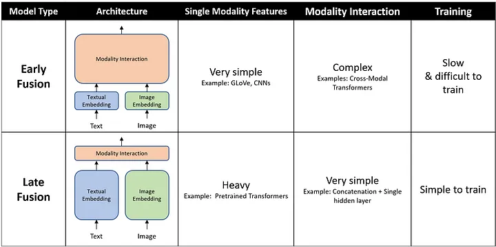
Fig 4: Multimodal Fusion for VQA [14]
Two common approaches for multimodal fusion are (i) concatenation + linear projection, or (ii) cross-attention.
Decoder
A language decoder (e.g., GPT-2) generates the answer token-by-token from the fused representation:
\[P(s|\mathbf{F}) = \prod_{t} P(s_t \mid s_{t}, \mathbf{F})\]Our VLM Model
Architecture
Following the general framework outlined above, we used the following pipeline:
- Text Encoder: BERT
- Image Encoder: ViT
- Fusion layer: FC + ReLU
- Language Model: GPT2
Vision Encoder
We utilize Vision Transformer (ViT) as the backbone for image feature extraction. ViT splits images into patches and applies the Transformer architecture directly to these patches, enabling efficient computation and scalability. The encoder outputs a high-dimensional feature vector representing the image.
Model Used: google/vit-base-patch16-224
Text Encoder
For the text encoder, we use BERT (Bidirectional Encoder Representations from Transformers). BERT generates a contextual embedding for the question by considering bidirectional relationships between words.
Model Used: bert-base-uncased
Multimodal Fusion
A fully connected layer is used to combine the vision and text embeddings. The fused representation enables the decoder to utilize both modalities effectively.
Language Decoder
The GPT-2 language model generates the natural language response. The decoder takes the fused multimodal embeddings as input and produces the answer in a token-by-token manner.
Model Used: GPT-2
Implementation Details
The VQA model is implemented in PyTorch using the Transformers library. Key steps:
Preprocessing:
Images are resized and converted into tensor format using a feature extractor.
Questions are tokenized into embeddings.
Forward Pass:
Vision and text features are extracted using ViT and BERT.
Features are fused using a linear layer.
The fused embeddings are passed into GPT-2 for answer generation.
Results
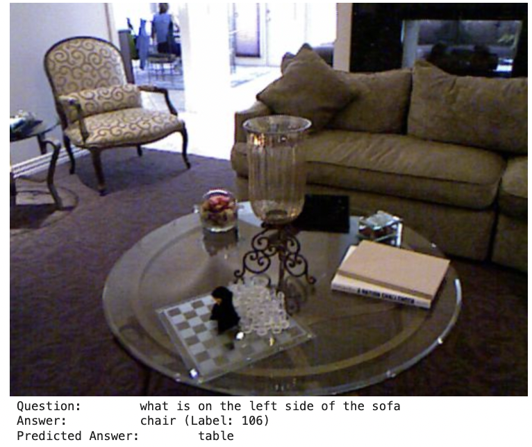
Currently, the model is in its basic implementation phase. Preliminary results indicate that the architecture is functional, with generated answers being syntactically coherent but requiring fine-tuning for better accuracy.
Below are some example results of the VQA model on test images. Each image includes the question, the ground-truth answer, and the model’s predicted answer.
| Example 1 | Example 2 | Example 3 | Example 4 | Example 5 |
|---|---|---|---|---|
 |
||||
| {: style=”border: 1px;”} {: style=”width: 200px; max-width: 100%;”} | 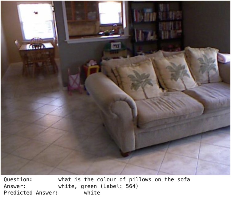 |
|||
| {: style=”border: 1px;”} {: style=”width: 200px; max-width: 100%;”} | 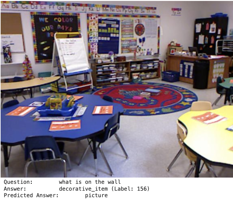 |
|||
| {: style=”border: 1px;”} {: style=”width: 200px; max-width: 100%;”} | 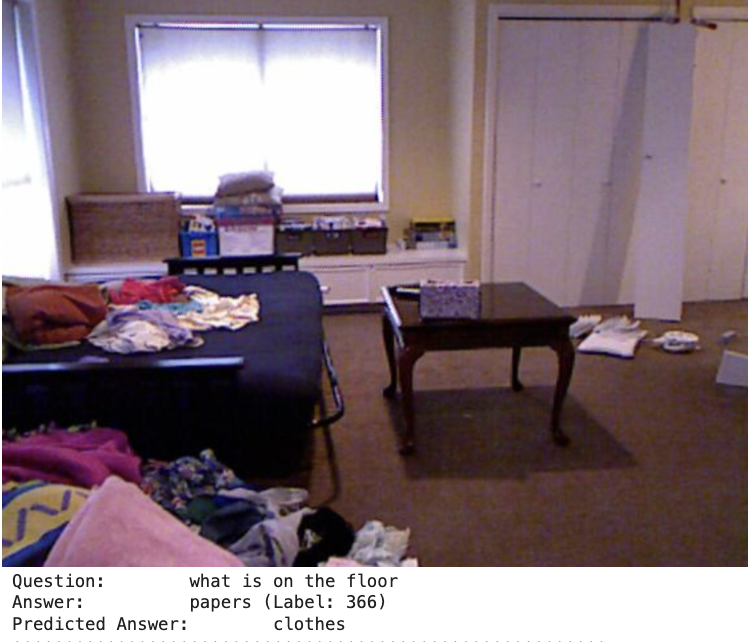 |
|||
| {: style=”border: 1px;”} {: style=”width: 200px; max-width: 100%;”} | 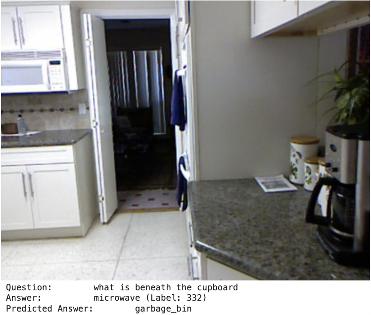 |
|||
| {: style=”border: 1px;”} {: style=”width: 200px; max-width: 100%;”} |
Fig 5: Model question & predicted answer pairs.
Future Work
-
Fine-Tuning: Train the model on a large-scale VQA dataset for improved performance.
-
Augmented VQA: Integrate semantic similarity metrics like Wu-Palmer similarity for robust evaluation.
-
Model Optimization: Experiment with advanced fusion techniques and larger language models.
-
Benchmarks: Evaluate on standard datasets such as VQA v2 and GQA.
Code
Training Curves
For more training curves check out wandb: https://wandb.ai/music123/huggingface?nw=nwuserrs545837
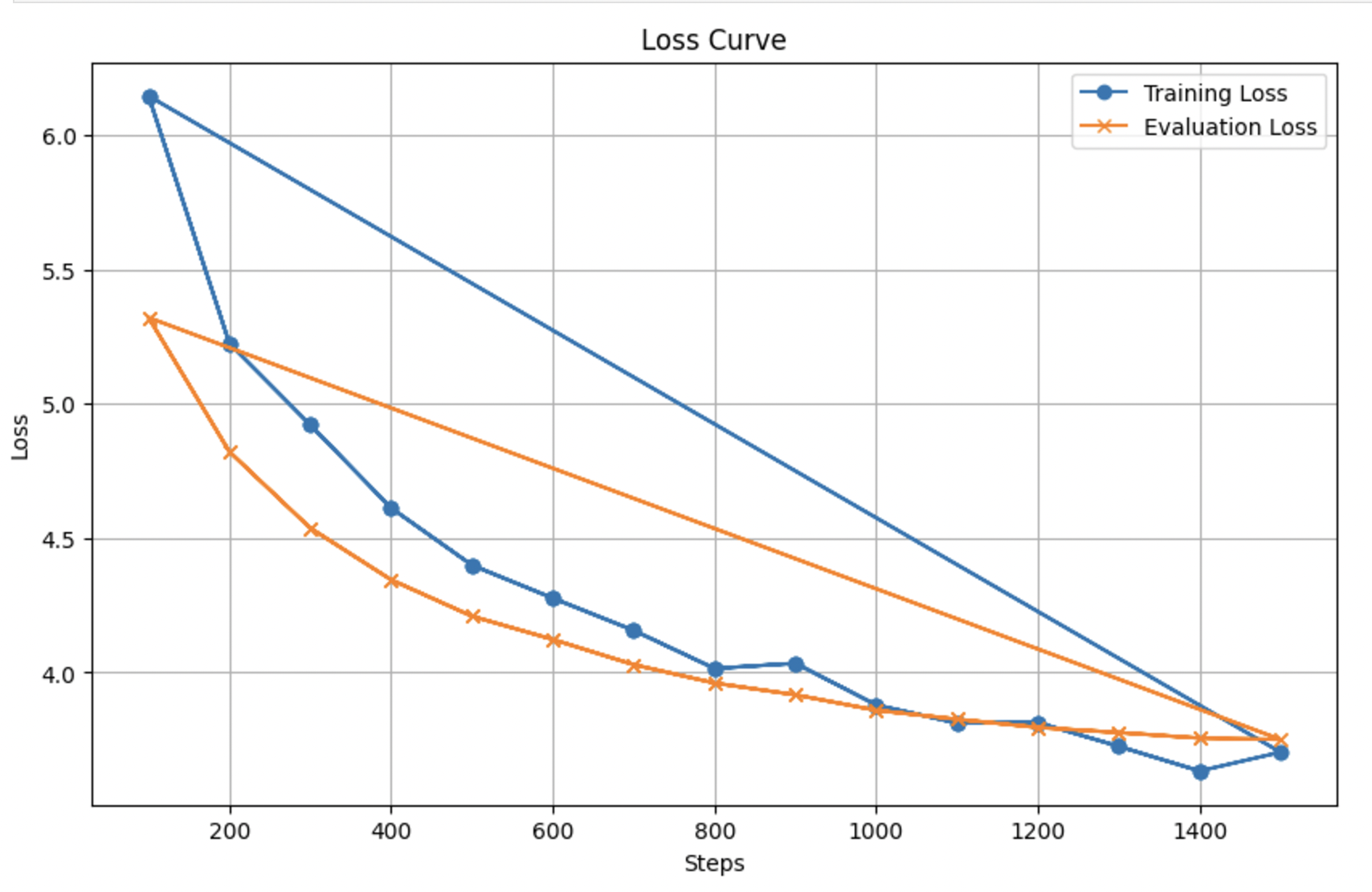
Fig 6: Training Curve for Our Model
Idefics3
Motivation
The Idefics3 model was chosen due to its robust performance across diverse benchmarks. Specifically, it was chosen since:
- State of the Art: Idefics3 is considered state-of-the-art for multiple benchmarks.
- Efficiency: Idefics3 is a lightweight model that is efficient to train and deploy.
- Open Domain Tasks: Idefics3 is able to perform well on open domain tasks such as VQA as well as closed domain tasks (e.g. MCQs) showing its versatility.
Architecture
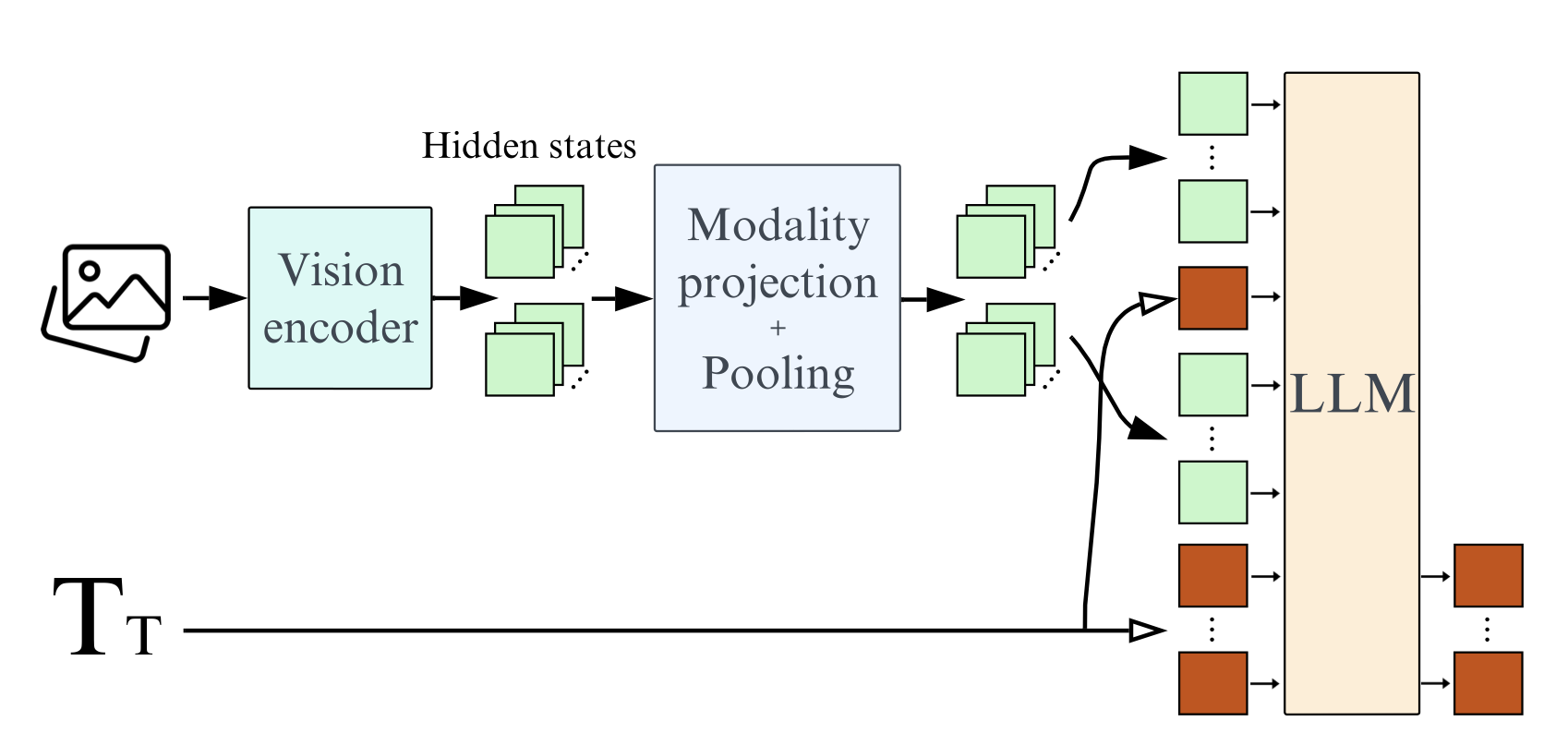
Fig 7: Idefics3 Architecture [11].
- Vision Encoder: The model uses the SigLIP-SO400M transformer as the vision encoder. The transformer is an open-source model developed by Google using the CLIP architecture with Sigmoid loss.
- LLM: The model uses Llama 3.1 Instruct as the language model. This is a big upgrade from Mistral 7B which is significantly outperformed by Llama 3.1.
- Pixel Shuffle: The model uses a pixel shuffle strategy to connect the vision encoder and the language model. This allows the model to enhance its OCR abilities while acting as a pooling tecnique to reduce the number of hidden states in the model by a factor of 4.
Code
The Idefics3 model is publicly available on HuggingFace. To import the model,
from transformers import AutoProcessor, AutoModelForVision2Seq
import torch

model_name = "HuggingFaceM4/Idefics3-8B-Llama3"
model = AutoModelForVision2Seq.from_pretrained(model_name, torch_dtype=torch.float16)
processor = AutoProcessor.from_pretrained(model_name)
Once you have imported the model, you can use the following function to run inference on a text-image pair.
def run_inference(model, processor, image, text_prompt):
  inputs = processor(
    images=image,
    text=text_prompt,
    return_tensors="pt"
    ).to("cuda", torch.float16)
  generated_ids = model.generate(**inputs)
  generated_text = processor.batch_decode(
    generated_ids,
    skip_special_tokens=True
    )[0].strip()
  return generated_text
Performance
Here is the performance of Idefics3 on some commonly used benchmarks:
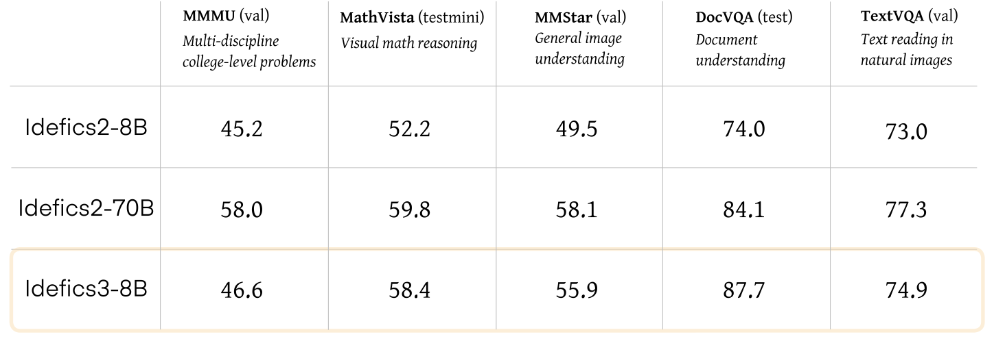
Fig 8: Idefics3 Performance [6].
LLAVA
Motivation
LLAVA is another robust, state of the art model capable of open-domain question answering. Specifically, it was selected due to:
- Visual Understanding: LLAVA is able to perform fine grained visual understanding such as recognizing small objects, or subtle attributes.
- Robust Multimodal Pretraining: LLAVA is trained on a vast dataset of text-image pairs, allowing to capture the semantic relationship between the image and the text.
Architecture
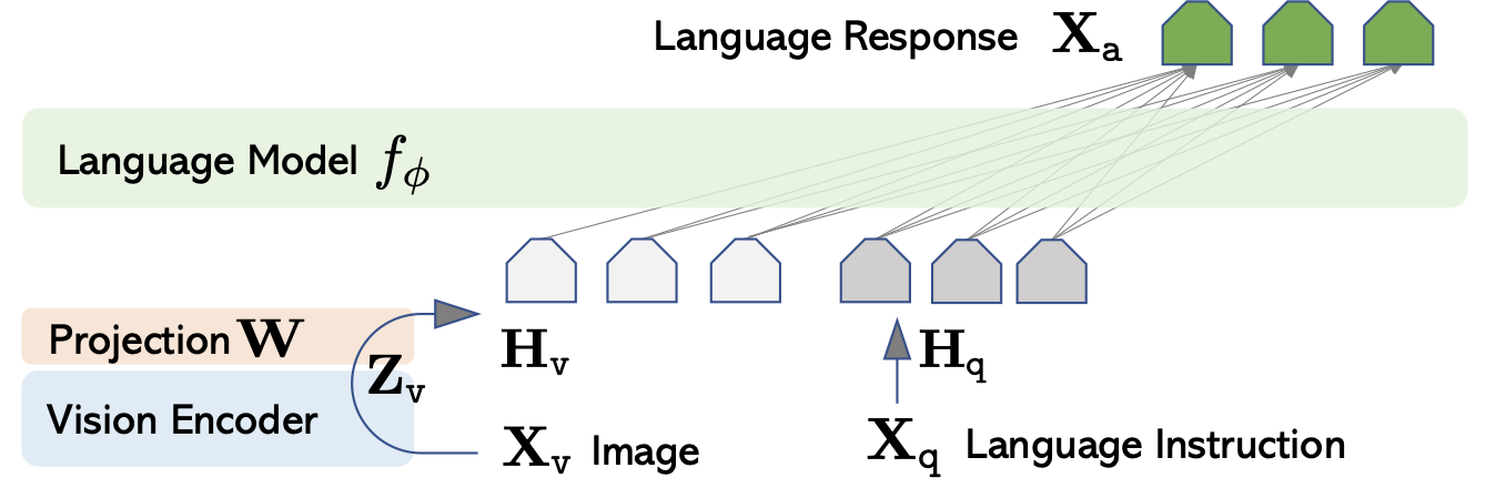
Fig 9: LLaVA Architecture [12].
- Vision Encoder: This model uses a pre-trained CLIP visual encoder ViT-L/14.
- Language Model: This model uses Vicuna due to its superior instruction following abilities.
- Linear Projection: The model uses a learnable linear projection to connect the image features to the word embedding space.
Code
Similar to Idefics3, LLaVA is also available on HuggingFace. Thus, LLaVA can be imported and run as follows:
from transformers import AutoProcessor, AutoModelForVision2Seq
import torch

model_name = "liuhaotian/llava-v1.6-vicuna-7b"
model = AutoModelForVision2Seq.from_pretrained(model_name, torch_dtype=torch.float16)
processor = AutoProcessor.from_pretrained(model_name)

def run_inference(model, processor, image, text_prompt):
  inputs = processor(
    images=image,
    text=text_prompt,
    return_tensors="pt"
    ).to("cuda", torch.float16)
  generated_ids = model.generate(**inputs)
  generated_text = processor.batch_decode(
    generated_ids,
    skip_special_tokens=True
    )[0].strip()
  return generated_text

# Example usage
image = Image.open("path/to/image.jpg")
text_prompt = "What is the color of the object in the image?"
result = run_inference(model, processor, image, text_prompt)
print(result)
Performance
| Version | LLM | Schedule | Checkpoint | MMMU | MathVista | VQAv2 | GQA | VizWiz | SQA | TextVQA | POPE | MME | MM-Bench | MM-Bench-CN | SEED-IMG | LLaVA-Bench-Wild | MM-Vet | |———-|———-|———–|———–|—|—|—|—|—|—|—|—|—|—|—|—|—|—| | LLaVA-1.6 | Vicuna-7B | full_ft-1e | liuhaotian/llava-v1.6-vicuna-7b | 35.8 | 34.6 | 81.8 | 64.2 | 57.6 | 70.1 | 64.9 | 86.5 | 1519/332 | 67.4 | 60.6 | 70.2 | 81.6 | 43.9 | | LLaVA-1.6 | Vicuna-13B | full_ft-1e | liuhaotian/llava-v1.6-vicuna-13b | 36.2 | 35.3 | 82.8 | 65.4 | 60.5 | 73.6 | 67.1 | 86.2 | 1575/326 | 70 | 64.4 | 71.9 | 87.3 | 48.4 | | LLaVA-1.6 | Mistral-7B | full_ft-1e | liuhaotian/llava-v1.6-mistral-7b | 35.3 | 37.7 | 82.2 | 64.8 | 60.0 | 72.8 | 65.7 | 86.7 | 1498/321 | 68.7 | 61.2 | 72.2 | 83.2 | 47.3 | | LLaVA-1.6 | Hermes-Yi-34B | full_ft-1e | liuhaotian/llava-v1.6-34b | 51.1 | 46.5 | 83.7 | 67.1 | 63.8 | 81.8 | 69.5 | 87.7 | 1631/397 | 79.3 | 79 | 75.9 | 89.6 | 57.4 |
Credits: https://github.com/haotian-liu/LLaVA/blob/main/
Evaluation Benchmarks
Benchmarks
In order to evaluate the models, we chose 3 datasets that collectively address different aspects of VQA: VQAv2 for general VQA, OK-VQA for visual reasoning using outside knowledge, and MATH-VQA for mathematical and logical reasoning. The choice of models result in a robust and comprehensive evaluation of the models.
VQAv2
Motivation: VQAv2 is a widely used dataset for VQA, often considered as the baseline for VQA models. It emphasizes image and linguistic understanding while eliminating linguistic biases.
Specifications:
- Contains ~1.1 million questions with ~13 million associated answers based on images from the COCO dataset.
- Creates a balanced dataset using the following method: “given an (image, question, answer) triplet (I , Q, A) from the VQA dataset, we ask a human subject to identify an image I′ that is similar to I but results in the answer to the question Q to become A′ (which is different from A).”[7]
Examples:
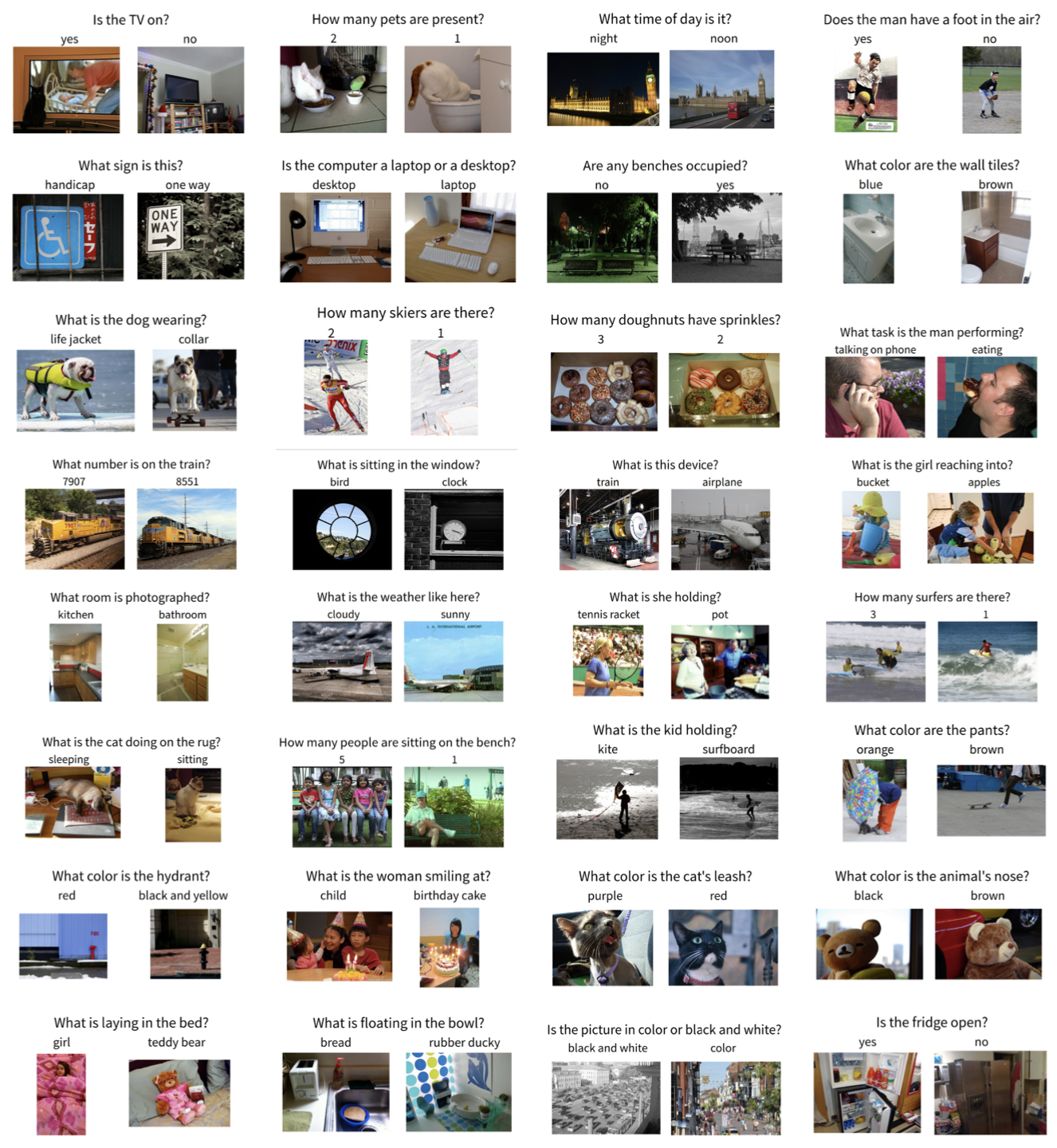
Fig 10: VQAv2 Examples [7].
OK-VQA
Motivation: Current VQA datasets favor image recognition and simple questions such as counting or identifying colors. However, real-world VQA tasks require reasoning using information from outside the image or question domain. OK-VQA addresses this by creating a dataset that requires reasoning using information from outside the image or question domain.
Specification:
- Contains 14,055 questions with 14,031 answers using images from the COCO dataset.
Answering OK-VQA questions is a challeng- ing task since, in addition to understanding the question and the image, the model needs to: (1) learn what knowledge is necessary to answer the questions, (2) determine what query to do to retrieve the necessary knowledge from an outside source of knowledge, and (3) incorporate the knowledge from its original representation to answer the question.[13]
Examples:
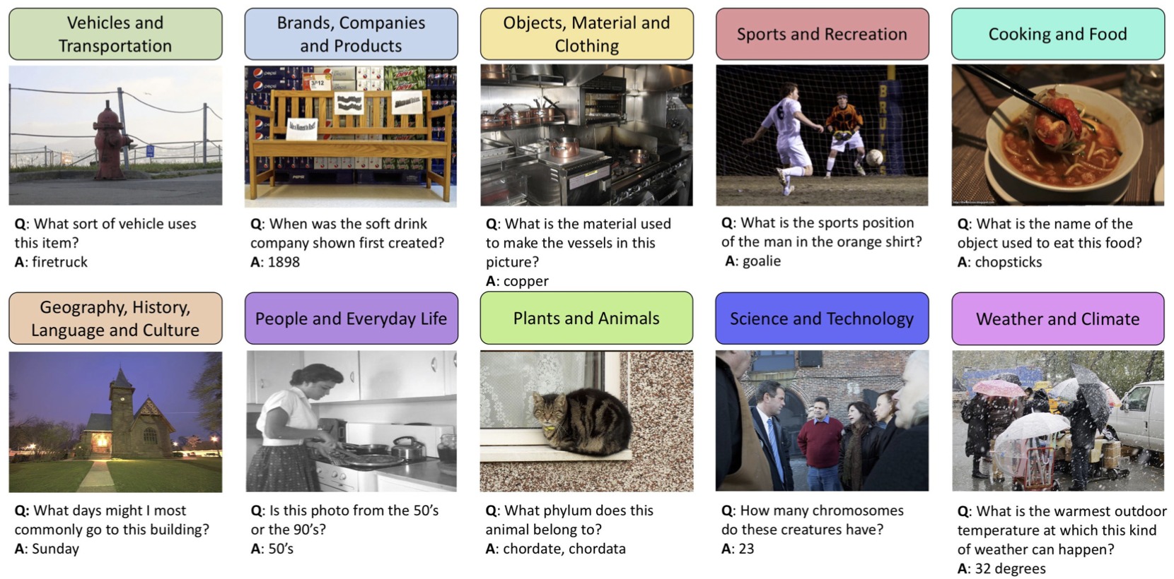
Fig 11: OK-VQA Examples [13].
MATH-VQA
Motivation: This dataset tests the mathematical reasoning ability of a model as compared to an average human. It provides a broad and diverse dataset of questions testing the mathematical reasoning ability of models.
Specifications:
- Contains 3,040 questions using 3,472 unique images providing mathematical context.
- Questions are categorized into 5 difficult levels and 16 distinct mathematical disciplines.
Examples:
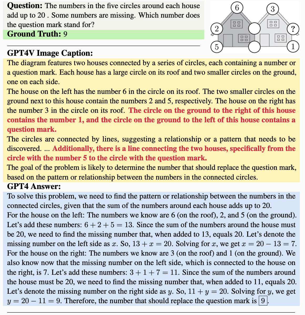
Fig 12: MATH-VQA Examples [17].
Augmented VQA
Standard datasets are excellent benchmarks for evaluating baseline performance. However, real-world applications often involve noisy and distorted visual inputs, making robustness critical. To address this, we created A-VQA, an augmented version of VQAv2 using a variety of augmentation techniques inspired by Ishmam et al. (2024) [6].
Augmentation Techniques
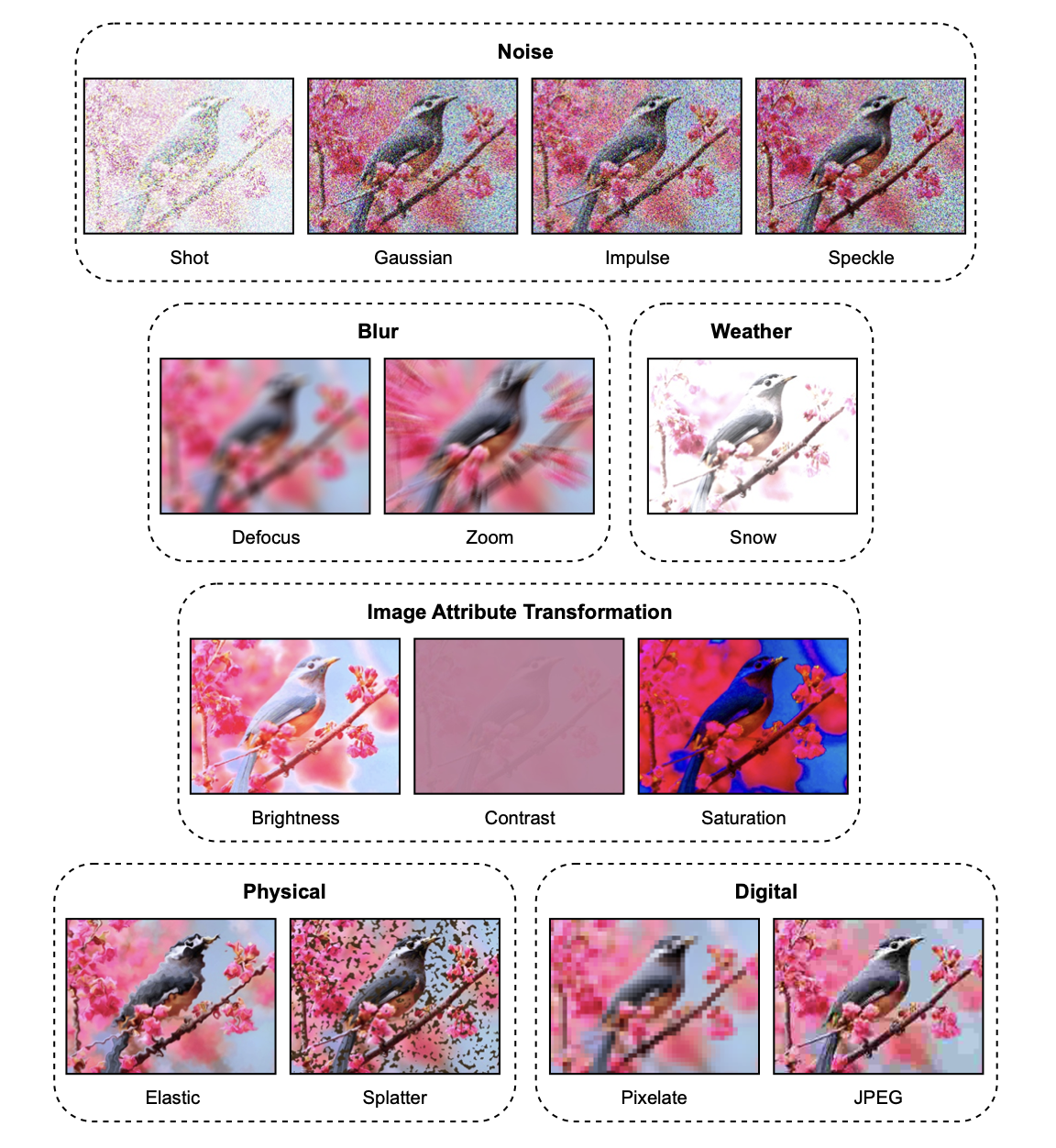
Fig 13: Augmentation Techniques [6].
The above image shows the augmentation techniques implemented in Ishmam et al. (2024) [6]. For our A-VQA dataset, we implemented the following augmentation techniques:
Noise Augmentation
- Shot Noise: Also called Poisson Noise, this technique adds noise to the image using a Poisson distribution.
def __shot_noise(self): """Credits: https://github.com/ishmamt/VQA-Visual-Robustness-Benchmark/blob/master/generator.py""" c = [.08, .2, 0.5, 0.8, 1.2][self.factor - 1] x = np.array(self.image) / 255. new_img= np.clip(x+(np.random.poisson( size=x.shape, lam=c)), 0, 1) * 255 new_img=np.float32(new_img) return cv2.cvtColor(new_img, cv2.COLOR_BGR2RGB) - Gaussian Noise: This technique adds noise to the image using a Gaussian distribution.
def __gaussian_noise(self): """Credits: https://github.com/ishmamt/VQA-Visual-Robustness-Benchmark/blob/master/generator.py""" c = [.08, .12, 0.18, 0.26, 0.38][self.factor - 1] x = np.array(self.image) / 255. new_img= np.clip(x+(np.random.normal(size=x.shape, scale=c)), 0, 1) * 255 new_img=np.float32(new_img) return (cv2.cvtColor(new_img, cv2.COLOR_BGR2RGB)) - Impulse Noise: This technique adds noise to the image by adding random isolated pixels with contrasting values to an image simulating the “salt and pepper” noise.
def __speckle_noise(self): """Credits: https://github.com/ishmamt/VQA-Visual-Robustness-Benchmark/blob/master/generator.py""" c = [.15, .2, 0.35, 0.45, 0.6][self.factor - 1] x = np.array(self.image) / 255. return (cv2.cvtColor(np.float32(np.clip(x + x * np.random.normal(size=x.shape, scale=c), 0, 1) * 255), cv2.COLOR_BGR2RGB)) - Speckle Noise: Uses a uniform distribution to change the pixel values in the image to add noise.
def __impulse_noise(self):
  """Credits: https://github.com/ishmamt/VQA-Visual-Robustness-Benchmark/blob/master/generator.py"""
  c = [.03, .06, .09, 0.17, 0.27][self.factor - 1]
  x = sk.util.random_noise(np.array(self.image) / 255., mode='s&p', amount=c)
  return (cv2.cvtColor(np.float32(np.clip(x, 0, 1) * 255), cv2.COLOR_BGR2RGB))
Blur Augmentation
- Defocus Blur: Uses channel-wise convolution to simulate the blurring effect of a camera lens when the subject is out of focus. ```python def __defocus_blur(self): “"”Credits: https://github.com/ishmamt/VQA-Visual-Robustness-Benchmark/blob/master/generator.py””” c = [(3, 0.1), (4, 0.5), (6, 0.5), (8, 0.5), (10, 0.5)][self.factor - 1] x = np.array(self.image) / 255. kernel = self.disk(radius=c[0], alias_blur=c[1])
channels = [] for d in range(3): channels.append(cv2.filter2D(x[:, :, d], -1, kernel)) channels = np.array(channels).transpose((1, 2, 0)) # 3x224x224 -> 224x224x3 return (cv2.cvtColor(np.float32(np.clip(channels, 0, 1) * 255), cv2.COLOR_BGR2RGB))
2. **Zoom Blur**: Uses clipping with a zoom factor to simulate the zoom blurring effect in cameras due to rapid camera motion towards the subject.
```python
def __zoom_blur(self):
  """Credits: https://github.com/ishmamt/VQA-Visual-Robustness-Benchmark/blob/master/generator.py"""
  c = [np.arange(1, 1.11, 0.01),
        np.arange(1, 1.16, 0.01),
        np.arange(1, 1.21, 0.02),
        np.arange(1, 1.26, 0.02),
        np.arange(1, 1.31, 0.03)][self.factor - 1]
  x = (np.array(self.image) / 255.).astype(np.float32)
  out = np.zeros_like(x)
  for zoom_factor in c:
      temp = self.__clipped_zoom(x, zoom_factor)
      out += temp


  x = (x + out) / (len(c) + 1)
  return (cv2.cvtColor(np.float32(np.clip(x, 0, 1) * 255), cv2.COLOR_BGR2RGB))
- Glass Blur: Uses a Gaussian filter to simulate the apperance of an object when viewed through a frosted glass. ```python def __glass_blur(self): c = [(0.7, 1, 2), (0.9, 2, 1), (1, 2, 3), (1.1, 3, 2), (1.5, 4, 2)][self.factor - 1] x = np.uint8(gaussian(np.array(self.image) / 255., sigma=c[0], channel_axis=-1) * 255)
# locally shuffle pixels for i in range(c[2]): for h in range(x.shape[0] - c[1], c[1], -1): for w in range(x.shape[1] - c[1], c[1], -1): dx, dy = np.random.randint(-c[1], c[1], size=(2,)) h_prime, w_prime = h + dy, w + dx # swap x[h, w], x[h_prime, w_prime] = x[h_prime, w_prime], x[h, w]
return (cv2.cvtColor(np.float32(np.clip(gaussian(x / 255., sigma=c[0], channel_axis=-1), 0, 1) * 255), cv2.COLOR_BGR2RGB))
##### Attribute Transformations
1. **Brightness Transform**: Converts the image from RGB to HSV and then adjusts the value channel.
```python
def __brightness_transform(self):
  """Credits: https://github.com/ishmamt/VQA-Visual-Robustness-Benchmark/blob/master/generator.py"""
  c = [.1, .2, .3, .4, .5][self.factor - 1]
  x = np.array(self.image) / 255.
  x = sk.color.rgb2hsv(x)
  x[:, :, 2] = np.clip(x[:, :, 2] + c, 0, 1)
  x = sk.color.hsv2rgb(x)
  return (cv2.cvtColor(np.float32(np.clip(x, 0, 1) * 255), cv2.COLOR_BGR2RGB))
- Contrast Transform: Clamped output of a linear transformation of the image using the mean pixel intensity gives a contrast transform.
def __contrast_transform(self): """Credits: https://github.com/ishmamt/VQA-Visual-Robustness-Benchmark/blob/master/generator.py""" c = [0.4, .3, .2, .1, .05][self.factor - 1] x = np.array(self.image) / 255. means = np.mean(x, axis=(0, 1), keepdims=True) return (cv2.cvtColor(np.float32(np.clip((x - means) * c + means, 0, 1) * 255), cv2.COLOR_BGR2RGB)) - Saturation Transform: Implementation converts the image from RGB to HSV and then adjusts the saturation channel.
def __saturation_transform(self):
  """Credits: https://github.com/ishmamt/VQA-Visual-Robustness-Benchmark/blob/master/generator.py"""
  c = [(0.3, 0), (0.1, 0), (2, 0), (5, 0.1), (20, 0.2)][self.factor - 1]
  x = np.array(self.image) / 255.
  x = sk.color.rgb2hsv(x)
  x[:, :, 1] = np.clip(x[:, :, 1] * c[0] + c[1], 0, 1)
  x = sk.color.hsv2rgb(x)
  return (cv2.cvtColor(np.float32(np.clip(x, 0, 1) * 255), cv2.COLOR_BGR2RGB))
Physical Transformations
- Elastic Transform: Simulates the effect of stretching or wrapping the image. ```python def __elastic_transform(self): “"”Credits: https://github.com/ishmamt/VQA-Visual-Robustness-Benchmark/blob/master/generator.py””” c = [(244 * 2, 244 * 0.7, 244 * 0.1), # 244 should have been 224, but ultimately nothing is incorrect (244 * 2, 244 * 0.08, 244 * 0.2), (244 * 0.05, 244 * 0.01, 244 * 0.02), (244 * 0.07, 244 * 0.01, 244 * 0.02), (244 * 0.12, 244 * 0.01, 244 * 0.02)][self.factor - 1]
image = np.array(self.image, dtype=np.float32) / 255. shape = image.shape shape_size = shape[:2]
# random affine center_square = np.float32(shape_size) // 2 square_size = min(shape_size) // 3 pts1 = np.float32([center_square + square_size, [center_square[0] + square_size, center_square[1] - square_size], center_square - square_size]) pts2 = pts1 + np.random.uniform(-c[2], c[2], size=pts1.shape).astype(np.float32) M = cv2.getAffineTransform(pts1, pts2) image = cv2.warpAffine(image, M, shape_size[::-1], borderMode=cv2.BORDER_REFLECT_101)
dx = (gaussian(np.random.uniform(-1, 1, size=shape[:2]), c[1], mode=’reflect’, truncate=3) * c[0]).astype(np.float32) dy = (gaussian(np.random.uniform(-1, 1, size=shape[:2]), c[1], mode=’reflect’, truncate=3) * c[0]).astype(np.float32) dx, dy = dx[…, np.newaxis], dy[…, np.newaxis]
x, y, z = np.meshgrid(np.arange(shape[1]), np.arange(shape[0]), np.arange(shape[2])) indices = np.reshape(y + dy, (-1, 1)), np.reshape(x + dx, (-1, 1)), np.reshape(z, (-1, 1)) return (cv2.cvtColor(np.float32(np.clip(map_coordinates(image, indices, order=1, mode=’reflect’).reshape(shape), 0, 1) * 255), cv2.COLOR_BGR2RGB))
2. **Splatter Transform**: Simulates the effect of splattering paint or any other liquid on the image.
```python
def __spatter_transform(self):
  """Credits: https://github.com/ishmamt/VQA-Visual-Robustness-Benchmark/blob/master/generator.py"""
  c = [(0.65, 0.3, 4, 0.69, 0.6, 0),
        (0.65, 0.3, 3, 0.68, 0.6, 0),
        (0.65, 0.3, 2, 0.68, 0.5, 0),
        (0.65, 0.3, 1, 0.65, 1.5, 1),
        (0.67, 0.4, 1, 0.65, 1.5, 1)][self.factor - 1]
  x = np.array(self.image, dtype=np.float32) / 255.

  liquid_layer = np.random.normal(size=x.shape[:2], loc=c[0], scale=c[1])

  liquid_layer = gaussian(liquid_layer, sigma=c[2])
  liquid_layer[liquid_layer < c[3]] = 0
  if c[5] == 0:
      liquid_layer = (liquid_layer * 255).astype(np.uint8)
      dist = 255 - cv2.Canny(liquid_layer, 50, 150)
      dist = cv2.distanceTransform(dist, cv2.DIST_L2, 5)
      _, dist = cv2.threshold(dist, 20, 20, cv2.THRESH_TRUNC)
      dist = cv2.blur(dist, (3, 3)).astype(np.uint8)
      dist = cv2.equalizeHist(dist)
      ker = np.array([[-2, -1, 0], [-1, 1, 1], [0, 1, 2]])
      dist = cv2.filter2D(dist, cv2.CV_8U, ker)
      dist = cv2.blur(dist, (3, 3)).astype(np.float32)

      m = cv2.cvtColor(liquid_layer * dist, cv2.COLOR_GRAY2BGRA)
      m /= np.max(m, axis=(0, 1))
      m *= c[4]

      # water is pale turqouise
      color = np.concatenate((175 / 255. * np.ones_like(m[..., :1]),
                              238 / 255. * np.ones_like(m[..., :1]),
                              238 / 255. * np.ones_like(m[..., :1])), axis=2)

      color = cv2.cvtColor(color, cv2.COLOR_BGR2BGRA)
      x = cv2.cvtColor(x, cv2.COLOR_BGR2BGRA)

      return (cv2.cvtColor(np.clip(x + m * color, 0, 1), cv2.COLOR_BGRA2RGB) * 255)
  else:
      m = np.where(liquid_layer > c[3], 1, 0)
      m = gaussian(m.astype(np.float32), sigma=c[4])
      m[m < 0.8] = 0

      # mud brown
      color = np.concatenate((63 / 255. * np.ones_like(x[..., :1]),
                              42 / 255. * np.ones_like(x[..., :1]),
                              20 / 255. * np.ones_like(x[..., :1])), axis=2)

      color *= m[..., np.newaxis]
      x *= (1 - m[..., np.newaxis])

      return (cv2.cvtColor(np.float32(np.clip(x + color, 0, 1) * 255), cv2.COLOR_BGR2RGB))
Digital Transformations
- Pixel Transform: Using downsampling and upsampling using bilinear interpolation, we are able to simulate a mosaic-like appearance.
def __pixelate_transform(self): """Credits: https://github.com/ishmamt/VQA-Visual-Robustness-Benchmark/blob/master/generator.py""" c = [0.6, 0.5, 0.4, 0.3, 0.15][self.factor - 1] x = np.array(self.image) # x = cv2.cvtColor(x, cv2.COLOR_BGR2RGB) width = int(x.shape[1] * c) height = int(x.shape[0] * c) dim = (width, height) resized = cv2.resize(x, dim, interpolation = cv2.INTER_AREA) return (cv2.cvtColor(np.float32(resized), cv2.COLOR_BGR2RGB)) - JPEG Compression: Simulates the effect of JPEG compression loss on the image.
def __jpeg_compression_transform(self):
  """Credits: https://github.com/ishmamt/VQA-Visual-Robustness-Benchmark/blob/master/generator.py"""
  c = [25, 18, 15, 10, 7][self.factor - 1]
  x = np.array(self.image)
  cv2.imwrite("temp.jpg", x, [int(cv2.IMWRITE_JPEG_QUALITY), c])
  temp = imread("temp.jpg")
  return temp
Note: Due to computational constraints, each dataset we use contains a random sample of 20 questions from the original dataset. Also, all the transforms have a severity factor that ranges from 1 to 5. We will be testing the models on each of the factors.
Wu-Palmer Similarity
VQA tasks often involve semantically close answers. For instance:
- Predicted answer: “car”
- Ground-truth answer: “vehicle”.
Exact-match scoring would return incorrect here, but WPS, derived from the WordNet lexical hierarchy, scores based on the semantic distance between terms.
Technical Details
WUPS is calculated as:
\[\text{WUPS}(x, y) = \frac{2 \cdot \text{Depth}(LCS(x, y))}{\text{Depth}(x) + \text{Depth}(y)}\]where:
- ( LCS(x, y) ): Longest Common Subsequence of ( x ) and ( y ) in the WordNet tree.
- Depth: Distance from the root node in the WordNet hierarchy.
Societal Impact & Applications
Due to the open-endedness of the VQA task, many potential applications can be readily formulated for VQA models. Broadly speaking, VQA is a task for eliciting visual information from images and visual media more generally; in this sense, any activity that involves interpreting and extracting knowledge from a visual medium can be seen as a specific instance of VQA.
In particular, a key application of VQA (even cited back when the task was first introduced in 2015 [2]) lies in interfaces for the visually impaired. Currently, visually impaired users have limited means of accessing and interacting with image-based content online. Although image captioning and similar methods have partially bridged this gap, current interfaces for visually impaired users lack the ability to make open-ended queries regarding images. In the future, VQA models may be able to provide this service and help visually impaired users engage with images and other forms of media online.
Conclusion
We began with a simple open-answer VQA framework and introduced advanced models (Idefics, LLAVA). Baseline models help understand the core pipeline, while cutting-edge architectures utilize instruction tuning, large LLMs, and alignment strategies to achieve superior results. Instruction tuning and semantic evaluation metrics (like WUP) advance VQA from brittle exact-match methods to more human-like reasoning.
Future Work
- Fine-Grained Reasoning: Better compositional understanding of scenes.
- Advanced Fusion: Employ more sophisticated cross-attention or hypercomplex layers.
- Evaluation: Incorporate richer semantic metrics (BERTScore, BLEU variants, human evaluation).
- Domain Adaptation: Specialize models to domains like medical or scientific imaging.
- Instruction & RLHF: Apply reinforcement learning from human feedback to further align models with user intent.
References
[1] Agrawal, A. et al. (2017). “VQA v2: Balanced Datasets for Visual Question Answering.” CVPR.
[2] Antol, S., Agrawal, A., Lu, J., Mitchell, M., Batra, D., Zitnick, C. L., & Parikh, D. (2015). Vqa: Visual question answering. In Proceedings of the IEEE international conference on computer vision (pp. 2425-2433).
[3] de Faria, Ana Cláudia Akemi Matsuki, et al. “Visual question answering: A survey on techniques and common trends in recent literature.” arXiv preprint arXiv:2305.11033 (2023).
[4] Devlin, J., Chang, M.-W., Lee, K., & Toutanova, K. (2019, May 24). Bert: Pre-training of deep bidirectional Transformers for language understanding. arXiv.org. https://arxiv.org/abs/1810.04805
[5] Dosovitskiy, A., Beyer, L., Kolesnikov, A., Weissenborn, D., Zhai, X., Unterthiner, T., Dehghani, M., Minderer, M., Heigold, G., Gelly, S., Uszkoreit, J., & Houlsby, N. (2021, June 3). An image is worth 16x16 words: Transformers for image recognition at scale. arXiv.org. https://arxiv.org/abs/2010.11929
[6] Farhan, Ishmam Md, et al. “Visual Robustness Benchmark for Visual Question Answering (VQA).” ArXiv (Cornell University), 3 July 2024, https://doi.org/10.48550/arxiv.2407.03386. Accessed 13 Dec. 2024.
[7] Goyal, Yash, et al. “Making the v in VQA Matter: Elevating the Role of Image Understanding in Visual Question Answering.” Computer Vision and Pattern Recognition, 1 July 2017, https://doi.org/10.1109/cvpr.2017.670. Accessed 21 Apr. 2023.
[8] Hudson, D. A., & Manning, C. D. (1970, January 1). GQA: A new dataset for real-world visual reasoning and compositional question answering. CVF Open Access. http://openaccess.thecvf.com/content_CVPR_2019/html/Hudson_GQA_A_New_Dataset_for_Real-World_Visual_Reasoning_and_Compositional_CVPR_2019_paper.html
[9] Kafle, Kushal, and Christopher Kanan. “An analysis of visual question answering algorithms.” Proceedings of the IEEE international conference on computer vision. 2017.
[10] Hugging Face Blog (2023). “Idefics: An Open-source Instruction-tuned Vision-Language Model.” https://huggingface.co/blog/idefics
[11] Laurençon, Hugo, et al. “Building and Better Understanding Vision-Language Models: Insights and Future Directions.” ArXiv (Cornell University), 22 Aug. 2024, https://doi.org/10.48550/arxiv.2408.12637. Accessed 13 Dec. 2024.
[12] Liu, Haotian, et al. “Visual Instruction Tuning.” ArXiv.org, 17 Apr. 2023, arxiv.org/abs/2304.08485.
[13] Marino, Kenneth, et al. “OK-VQA: A Visual Question Answering Benchmark Requiring External Knowledge.” ArXiv (Cornell University), 1 June 2019, https://doi.org/10.1109/cvpr.2019.00331. Accessed 11 Nov. 2023.
[14] Sahu, T. (2022, March 8). Visual question answering with Multimodal Transformers. Medium. https://medium.com/data-science-at-microsoft/visual-question-answering-with-multimodal-transformers-d4f57950c867
[15] Teney, D., Anderson, P., He, X., & van den Hengel, A. (1970, January 1). Tips and tricks for visual question answering: Learnings from the 2017 challenge. CVF Open Access. http://openaccess.thecvf.com/content_cvpr_2018/html/Teney_Tips_and_Tricks_CVPR_2018_paper.html
[16] Vaswani, A., Shazeer, N., Parmar, N., Uszkoreit, J., Jones, L., Gomez, A. N., Kaiser, Ł., & Polosukhin, I. (1970, January 1). Attention is all you need. Advances in Neural Information Processing Systems. https://proceedings.neurips.cc/paper/7181-attention-is-all-you-need - Radford, A. et al. (2018). “Improving Language Understanding by Generative Pre-Training.” OpenAI blog.
[17] Wang, Ke, et al. “Measuring Multimodal Mathematical Reasoning with MATH-Vision Dataset.” ArXiv (Cornell University), 22 Feb. 2024, https://doi.org/10.48550/arxiv.2402.14804.
[18] Wu, Zhibiao, and Martha Palmer. “Verb semantics and lexical selection.” arXiv preprint cmp-lg/9406033 (1994).