Medical image segmentation is a process that involves dividing a medical image into multiple distinct Regions of Interest corresponding to different organs, tissues, or pathological areas automatically. This technique allows healthcare professionals to interpret and analyze medical images like X-rays, ultrasounds, and CT scans much more efficiently than having to label areas by hand.

• Introduction
• Fully Convolutional Networks
  • Motivation
  • From Fully Connected to Fully Convolutional
  • Skip Connections
  • Performance
• U-Net
  • Motivation
  • Structure
  • Skip Connections
  • Training
  • Class Imbalance
  • Data Augmentation
  • Performance
• U-Net++
  • Motivation
  • Review of FCN and U-Net
  • Overview of Improvements
    • Re-designed Skip Pathways
    • Further Intuition
    • Deep Supervision
    • Results and Performance
• Running U-Net Codebase
  • Designing from Scratch
    • Encoder
    • Bottleneck:
    • Decoder:
    • Putting it all together
  • Find and Preprocessing Data
  • Training and Evaluating the Model
• References

Introduction

Medical image segmentation is a process that involves dividing a medical image into multiple distinct Regions of Interest corresponding to different organs, tissues, or pathological areas automatically. This technique allows healthcare professionals to interpret and analyze medical images like X-rays, ultrasounds, and CT scans much more efficiently than having to label areas by hand.

Traditional approaches to this problem include thresholding, graph partitioning, and clustering. While initially promising, innovations in deep learning and neural networks were able to take the technology to the next level. In this project, our goal is to explore how convolutional networks such as FCNs, U-Net, and U-Net++ have contributed to the development of segmentation as a computer vision field, and implement our own U-Net model for image segmentation.

Fully Convolutional Networks

Motivation

Fully Convolutional Networks (FCN), introduced by Long et al., are a class of neural networks designed for dense prediction tasks such as semantic segmentation [1]. FCNs, trained end-to-end and pixel-to-pixel, outperformed all previous segmentation approaches, and thus laid the foundations for future architectures such as U-Net to be developed for the more specialized task of medical image segmentation.

From Fully Connected to Fully Convolutional

Fully connected layers in neural networks were originally designed for tasks like image classification, that took an image as input and outputted a single classification label. For segmentation tasks, this approach poses many problems, such as loss of spatial information due to flattening and a fixed input size reducing the flexibility of the model. Fully convolutional networks completely eliminate fully connected layers, allowing the network to generate spatial feature maps after downsampling, which can then be upsampled up to the same image size.

FCNs adapt classifiers for dense prediction. Classification networks such as AlexNet use fully connected layers to take fixed-size inputs and produce nonspatial outputs, but the fully connected layers can also be viewed as convolutional layers whose kernel size matches the entire input region. This reinterpretation creates output maps for any input size, where the ground truth is available at every output cell. However, the output dimensions have still been reduced by subsampling, resulting in coarse output maps whose size has been reduced from the input by the pixel stride of the receptive fields of the output units.

To transform these coarse outputs back to dense pixels, we can also view upsampling with factor f as convolution with a fractional input stride of 1/f. Thus backwards convolution (aka transposed convolution) can be used with an output stride of f to upsample in-network, learning by backpropagation from the pixelwise loss [1]. The backwards convolution filter used does not need to have fixed weights as in traditional bilinear interpolation, but can instead be learned, further improving performance. This encoder(downsampling) and decoder (upsampling) architecture would continue to be refined later in U-Net and U-Net++.

Skip Connections

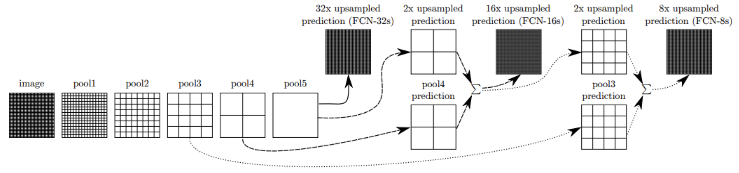
While existing architecture such as AlexNet and VGG can be modified to be fully convolutional and fine-tuned for segmentation, the resulting output is still somewhat coarse, caused by the 32 pixel stride at the final prediction layer limiting detail in the final output. FCNs mitigates this through introducing skip connections, which are links combining the final prediction layer with lower layers with less stride, illustrated in the figure below. The output stride can be divided in half by first predicting from pool4 with a 1x1 convolution layer, and summing this with the prediction obtained by adding a 2x upsampling layer to the stride 32 prediction. This net is called FCN-16s, while the network without skip connections is called FCN-32s [1]. This approach combines the final prediction result from the convolution layers’ high level semantic information with prediction results from an earlier layer’s low-level more detailed information for enhanced precision in the segmentation boundaries. Further optimization is made by summing predictions from pool3 with 2x upsampled predictions from the summed prediction used in FCN-16s and then 8x upsampling to build the net FCN8s.

Performance

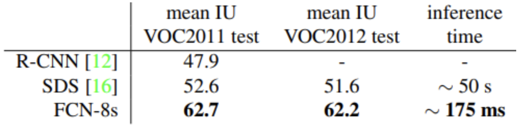
Existing methods at the time applying convnets to dense prediction problems did not train end-to-end and relied on either hybrid proposal-classifier models or used patchwise training, post-processing, or ensembles. These innovations allowed FCNs to recover more details in fine structures, separate closely interacting objects, and be robust against occlusion. Using fully convolutional layers through the entire network combined with skip connections allowed FCNs to outperform state of the art models at the time such as SDS in metrics like pixel accuracy, mean IoU, and inference time across multiple datasets.

U-Net

Motivation

U-Net, introduced by Ronneberger et al, is a convolutional neural network designed specifically for biomedical image segmentation [2]. U-Net iterates upon traditional convolution networks of purely classification and provides location information as well. Another challenge of biomedical imaging is due to the lack of data for training.

Structure

The name of U-Net originates from its U shaped structure. It has an encoder-decoder structure that has symmetric contracting and expanding paths.

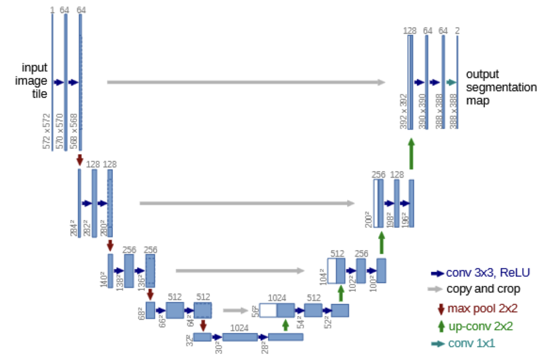
The bottleneck at the bottom of the U acts as a transition between encoder and decoder, which captures the most abstract and compressed representation of the image.

The expanding path (decoder) reconstructs the spatial resolution of the segmentation map while refining details using the high resolution features from the encoder. Each block begins with upsampling that doubles the spatial dimensions of the feature map.

Skip Connections

Skip connections in U-Net link feature maps from the encoder to the decoder. These connections allow the concatenation of high-resolution features from earlier layers in the encoder with the upsampled features in the decoder[2]. These Skip connections were originally introduced in the FCN architecture, discussed earlier. As a recap, they aided in the following:

• Recovering spatial information: Traditional convolutional networks suffered the progressive loss of spatial resolution due to repeated pooling and striding. Skip connections prevent this by reintroducing higher resolution feature maps directly.
• Improved boundary segmentation: biomedical images often have small and intricate structures, skip connections helped by combining localized information from earlier layers to global context from deeper layers.

Unlike other architectures such as FCN, U-Net uses concatenation instead of element-wise addition for its skip connections [2]. Concatenation helps preserve feature diversity by retaining all features from the encoder and decoder. This ensures both fine-grained encoder and upsampled decoder features are accessible for subsequent processing. Element-wise addition would discard/dilute unique information from each source, which is especially an issue if distributions differ significantly.

After concatenation, the decoder applies convolutional layers to combined feature maps that allows the network to learn optimal transformations that integrates spatial details and context.

Training

U-Net is trained using a pixel-wise cross-entropy loss. For an input \(x\), the output of the network is a probability distribution \(p_k(x)\) for each pixel. The soft-max is defined as

where \(a_k(x)\) denotes the activation value of class \(k\) at pixel \(x\), and \(K\) is the total number of classes[2].

The cross-entropy loss penalizes the deviation of the predicted probability \(p_{l(x)}(x)\) from the true class label \(l(x)\):

where \(w(x)\) is weight assigned to each pixel \(x\)[2].

Class Imbalance

In image segmentation tasks, problems with class imbalance in images is common, such as backgrounds taking up a large proportion of the image. This problem is especially apparent in biomedical segmentation tasks as class imbalance can exist across an entire dataset. U-Net introduces a pixel-wise weight map \(w(x)\) that assigns higher importance to underrepresented regions or specific boundaries

where \(w_c(x)\) balances class frequencies across the dataset, \(w_0\) and \(\sigma\) are constants controlling importance and spread of boundary weights, and \(d_1(x)\) and \(d_2(x)\) are distance of pixel \(x\) to the closest and second closest boundaries[2].

This encourages U-Net to focus on separating touching objects and improve segmentation performance at boundaries.

Data Augmentation

To overcome the limited amount of training data, U-Net also employs the following data augmentation techniques[2]:

• Elastic Deformations: simulate realistic distortions in tissue structure
• Rotations and Flips: ensures model invariance to orientation
• Intensity Variations: ensures network is robust to changes in image brightness and contrast

Performance

U-Net’s advantage over sliding-window CNNs came at its computation efficiency and delivering localization with global context instead of sacrificing one for the other.

The skip connections, class imbalance weight map, as well as data augmentation gave U-Net an edge over traditional FCNs as it was able to recover high-resolution features, improve segmentation accuracy, especially for boundary regions, as well as performing well in domains with limited data.

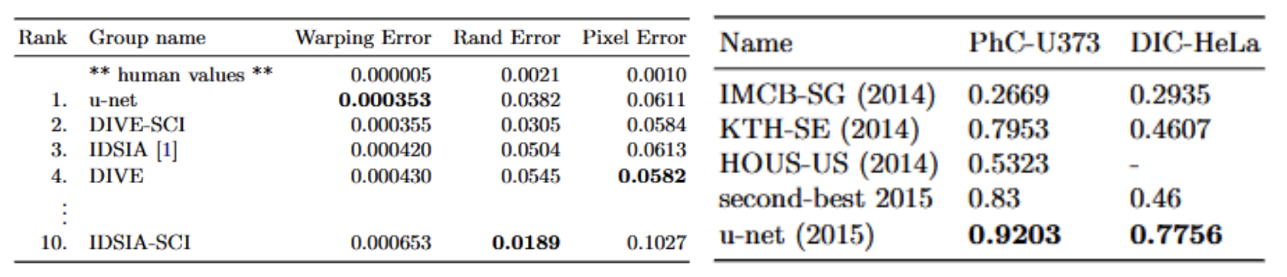
U-Net outperformed state of the art models at the time in metrics such as warping error and IoU scores on a variety of datasets.

U-Net++

Motivation

The original U-Net model was designed specifically for the purpose of biomedical image segmentation, winning several challenges at the ISBI (International Symposium on Biomedical Imaging) in 2015. However, in the world of medical imaging — where even the smallest errors could put the lives of patients at stake — the sense was that a model could never be good enough. It was with this in mind that U-Net++ was introduced, in a paper by Zhou et al., in an attempt to improve upon the base provided by U-Net.

Review of FCN and U-Net

The key idea behind both FCN and U-Net is the use of skip connections, an architecture originally proposed by Long et al. in the FCN paper.

In FCN, after the convolutional backbone (encoder) progressively downsamples the input image into a feature map, a small decoding process upsamples the map back to its original size. During the intermediate stages of the upsampling process, the authors used skip connections to pass “appearance information” from the final few encoding layers into the current feature representation. The addition of this information during the decoding process greatly improved segmentation results [1].

U-Net builds upon this by fully committing to the approach, creating a completely symmetrical encoder-decoder architecture where every single encoder layer passes its output to a corresponding decoder layer, rather than just the last few. They also change the operation behind the skip connections from element-wise addition to concatenation, which better preserves the separate components for processing [2].

Overview of Improvements

Re-designed Skip Pathways

UNet++ features a reimagining of skip connections. The main idea behind the change was to “bridge the semantic gap” between symmetrical encoder and decoder layers, before the fusion occured. It was thought that the learning task would become easier if the paired encoder and decoder feature maps were similar to each other.

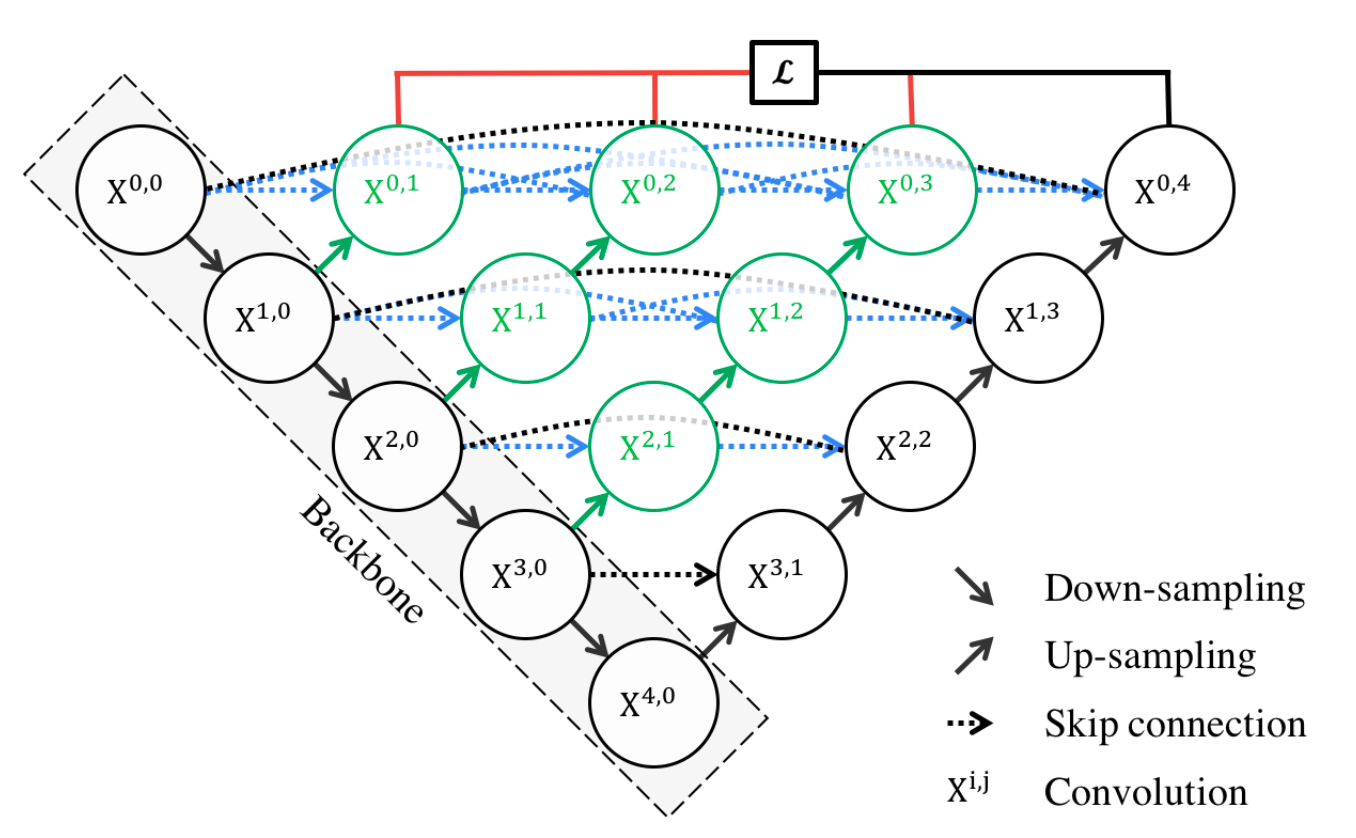
Above we see a diagram detailing the structure of UNet++. The black nodes on the left side represent the encoder, which extracts features from the input image by progressively down-sampling. Likewise, the black nodes on the right side represent the decoder. These nodes upsample feature maps to progressively increase spatial resolution and generate the final segmentation map at X^0,4 [3].

Nested dense skip pathways (blue and green arrows) connect encoder and decoder nodes, allowing feature maps to flow between layers and be progressively refined.

To make the connections clear, let’s dissect the mathematical formulation provided by the authors.

First, let’s define all of the notation. \(( x^{i,j} )\) denotes the output of node \(( X^{i,j} )\), as depicted in the diagram. The function \(( \mathcal{H}(.) )\) represents a convolution operation followed by an activation function. \(( \mathcal{U}(.) )\) represents an upsampling layer. The square brackets \(( [ \, ] )\) denote a concatenation layer [3].

We have two cases. The first occurs when \(( j = 0 )\), which indicates that our node belongs to the backbone encoder sub-network. In this scenario, the only input to our node \(( X^{i,0} )\) is the output from the previous encoder node, \(( X^{i-1,0} )\). We take this input and pass it through our convolution/activation operation \(( \mathcal{H} )\) to obtain the output \(( x^{i,0} )\) [3].

The second scenario is the general case when \(( j > 0 )\). For a node \(( X^{i,j} )\), we get the outputs from nodes \(( X^{i,0}, X^{i,1}, \dots, X^{i,j-1} )\), and concatenate them together, denoted as \(( [x^{i,0}, x^{i,1}, \dots, x^{i,j-1}] )\). Then, we take the output from node \(( x^{i+1,j-1} )\) and upsample it through \(( \mathcal{U} )\) (to match up its dimensions), before concatenating it to our result as well. We take this final concatenation of \(( j + 1 )\) outputs and run it through the convolution/activation operation \(( \mathcal{H} )\) to reduce feature depth and obtain the output \(( x^{i,j} )\) [3].

Further Intuition

With the mathematical formulation out of the way, we can try to think more intuitively about the skip connections. Let’s look at the node \(( X^{0,4} )\). In a classical U-Net model, it would receive inputs from \(( X^{1,3} )\) and \(( X^{0,0} )\), before concatenating them directly for further processing.

In Unet++, the process is no longer this simple. Instead, the re-designed skip connections make it so that both the encoder output \(( X^{0,0} )\) and the decoder output \(( X^{1,3} )\) are enriched with information from all of the other encoder states, shifting them “closer” semantically. Only then are they concatenated at \(( X^{0,4} )\).

Deep Supervision

The next feature introduced in UNet++ is deep supervision. Looking back at the model diagram, we can see the deep supervision component marked in red lines. Due to the intermediate nodes introduced by the nested skip pathways, we actually generate multiple, full resolution feature maps from \(( X^{0,1} )\), \(( X^{0,2} )\), \(( X^{0,3} )\), and \(( X^{0,4} )\) [3]. We can use \((1x1)\) convolutions to convert each of these feature maps into an full segmentation map, giving us four separate output maps to work with.

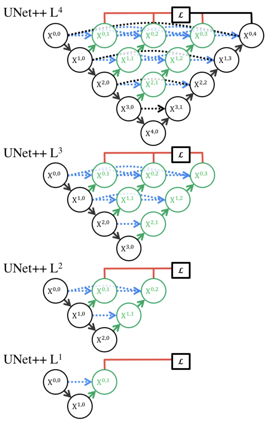
Each of these output maps corresponds to a “sub-model” of increasing depth: for example, \(( X^{0,1} )\) comes from a very shallow sub-model including just \(( X^{0,0} )\) and \(( X^{1,0} )\). On the other hand, \(( X^{0,4} )\) comes from the model in its entirety. The figure below illustrates this concept.

During training, we can choose to operate in “accurate mode”, where we average the losses from multiple predicted segmentation maps into one final loss. As for the loss itself, the authors opted for a combination of binary cross entropy loss and the DICE coefficient, shown below [3].

This is a batch loss, where we average the losses over all \(N\) training images in the batch.

On the other hand, during inference, a “fast mode” can be toggled where only one segmentation map is used as output: this provides several options, where selecting the output from a smaller, pruned sub-network decreases inference time significantly, at the cost of a small amount of accuracy [3].

Results and Performance

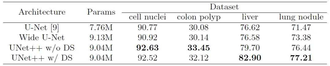
Unet++ was evaluated on datasets for four different tasks, including lung nodule segmentation, colon polyp segmentation, liver segmentation, and cell nuclei segmentation. Zhou et al. evaluated UNet++ against both a classical U-Net model, and a custom Wide U-Net model. The Wide U-Net results were used as a control, in order to ensure that the performance gain of UNet++ was not attributable purely to the increase in parameters [3].

Without deep supervision, UNet++ achieved an average IoU gain of 2.8 points and 3.3 points over U-Net and Wide U-Net, respectively. With deep supervision training, the gain increased to 3.9 and 3.4 points, respectively [3].

Running U-Net Codebase

Designing from Scratch

The original U-Net paper that we referenced did not provide the code that they used, so we had to create the U-Net model ourselves. We referenced the architecture they provided and followed the same design with an encoder, bottleneck, and decoder which calls for the following design

Input Image
    |
[Encoder] → (Conv + ReLU) → (Conv + ReLU) → Max Pooling → ...
    |
[Latent Layer] (Bottleneck)
    |
[Decoder] ← (Upconv + ReLU) ← (Concat with skip connections) → (Conv + ReLU) → ...
    |
Final Output (1x1 Conv) → (Softmax/Sigmoid)

Encoder

The encoder is built using two convolutional layers followed by a max-pooling operation at each step.

def double_conv_block(x, n_filters):
    x = layers.Conv2D(n_filters, 3, padding="same", activation="relu", kernel_initializer="he_normal")(x)
    x = layers.Conv2D(n_filters, 3, padding="same", activation="relu", kernel_initializer="he_normal")(x)
    return x

def downsample_block(x, n_filters):
    f = double_conv_block(x, n_filters)
    p = layers.MaxPool2D(2)(f)
    p = layers.Dropout(0.3)(p)
    return f, p

# Downsampling with the blocks
f1, p1 = downsample_block(inputs, 64)
f2, p2 = downsample_block(p1, 128)
f3, p3 = downsample_block(p2, 256)
f4, p4 = downsample_block(p3, 512)

Bottleneck:

   bottleneck = double_conv_block(p4, 1024)

Decoder:

def upsample_block(x, conv_features, n_filters):
   x = layers.Conv2DTranspose(n_filters, 3, 2, padding="same")(x)
   x = layers.concatenate([x, conv_features])
   x = layers.Dropout(0.3)(x)
   x = double_conv_block(x, n_filters)
   return x

   u6 = upsample_block(bottleneck, f4, 512)
   u7 = upsample_block(u6, f3, 256)
   u8 = upsample_block(u7, f2, 128)
   u9 = upsample_block(u8, f1, 64)
   outputs = layers.Conv2D(3, 1, padding="same", activation = "softmax")(u9)

Putting it all together

def build_unet():
   f1, p1 = downsample_block(inputs, 64)
   f2, p2 = downsample_block(p1, 128)
   f3, p3 = downsample_block(p2, 256)
   f4, p4 = downsample_block(p3, 512)
   bottleneck = double_conv_block(p4, 1024)
   u6 = upsample_block(bottleneck, f4, 512)
   u7 = upsample_block(u6, f3, 256)
   u8 = upsample_block(u7, f2, 128)
   u9 = upsample_block(u8, f1, 64)
   outputs = layers.Conv2D(3, 1, padding="same", activation = "softmax")(u9)
   unet_model = Model(inputs, outputs, name="U-Net")
   return unet_model

We referenced this video to help streamline the building process [4]

Find and Preprocessing Data

Before training the model, we first had to find a suitable database to use with annotated images and their corresponding segmentation masks. Instead of using medical imaging data, we decided to try something a bit different and instead worked with dogs. To do this, we referenced the Oxford-IIIT Pet Dataset [5] and only used annotated images of dogs. When it came to preprocessing the data, all we did was resize the images to have consistent dimensions, normalize them, as well downscale the data type from float64 to float32 for less computation. We also scaled the provided segmentation masks so that they would range from [0,2] instead of [1,3].

for _ in range(600):
    #Resize images and masks to 128x128
    images[_] = cv2.resize(images[_], (128, 128))
    masks[_] = cv2.resize(masks[_], (128, 128))

    #Normalize Images
    images[_] = images[_] / 255.0

    #Convert images from float64 to float32
    images[_] = images[_].astype(np.float32)

#Covert lists to np arrays so that we can scale the mask values to start at 0 instead of 1
images = np.array(images)
masks = np.array(masks)
#Scale the array
masks = masks - 1

We also split the data into 80% train and 20% test data.

Training and Evaluating the Model

Because of computational costs, we only trained the model for 10 epochs. Here are the results after training

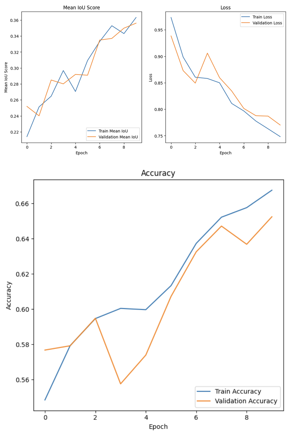
When testing our model, it performed somewhat well with an accuracy of 67.43% and a Mean IoU of 37.28%. We believe that the Mean IoU score is so low here due to the model’s poor performance when it came to detecting edges. Had we trained on more epochs, our model probably would have done better as the Mean IoU and accuracy curves are still increasing, and the loss is still decreasing.

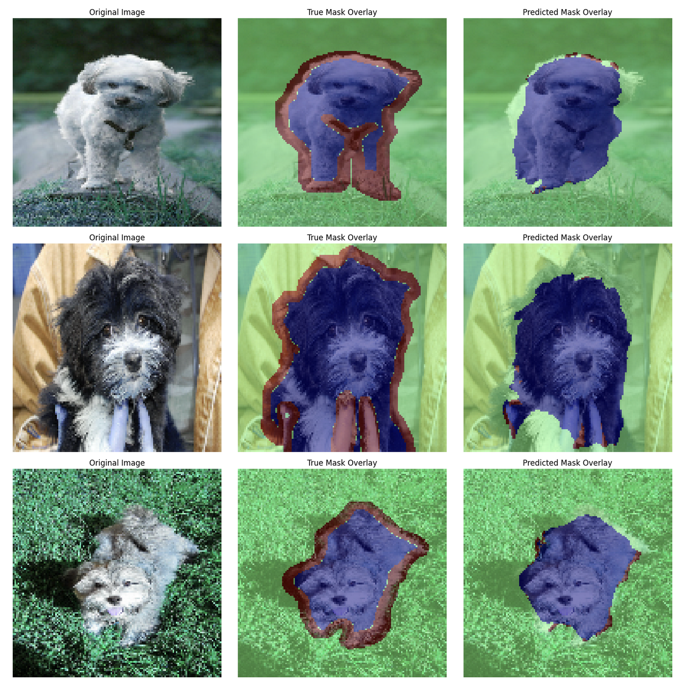
Above are some examples of segmentation maps created by our model. The green pixels are labeled as background, red pixels are border pixels, and the blue pixels are the dog we are trying to detect. As you can see, the model is still able to capture the general shape of the dogs and does a good job identifying the background, but struggles when it comes to identifying edges. We believe that our model would have performed much better in that regard had we trained for more epochs.

References

[1] Long, Jonathan, et al. “Fully Convolutional Networks for Semantic Segmentation.” Arxiv.org, 8 Mar 2015, https://arxiv.org/abs/1411.4038.

[2] Ronneberger, Olaf, et al. “U-Net: Convolutional Networks for Biomedical Image Segmentation.” Arxiv.org, 18 May 2015, https://arxiv.org/abs/1505.04597.

[3] Zhou, Zongwei, et al. “UNet++: A Nested U-Net Architecture for Medical Image Segmentation.” Arxiv.org, 18 Jul 2018, https://arxiv.org/abs/1807.10165

[4] Eran Feit. (2023, August 31). Creating an Animal Segmentation Model with U-Net and TensorFlow Keras. YouTube. https://www.youtube.com/watch?v=oHc4yrV64wU

[5] Parkhi, O. M., Vedaldi, A., Zisserman, A., & Jawahar, C. V. (2012). The Oxford Pets dataset University of Oxford. https://www.robots.ox.ac.uk/~vgg/data/pets/