Text Guided Image Generation

Text-guided image generation is an important milestone for both natural language procesing and computer vision. It seeks to use natural language prompts to generate new images or edit previous images. Recently diffusion models have been shown to produce better results than GANS in regards to text-guided image generation. In this article, we will be examining GLIDE: Towards Photorealistic Image Generation and Editing with Text-Guided Diffusion Models.

• Introduction
  • Video
• Background Architecture
  • Transformer Model for Text to Token Encoder
  • Diffusion Model
  • Classifier Free Guidance Loss Functions
  • Main Diffusion Model (ADM model architecture with additional text token residual connections)
  • Additional Upsampling Diffusion Model
  • Putting it All Together
• Training
  • Dataset
  • Training Process
• Evaluation
  • Results
• Demo
• Reference

Introduction

Video

Text-guided image generation is a natural fusion of computer vision and natural language processing. Advancements in text-guided image generation serve as important benchmarks in the development of both fields. Text-guided image generation seeks to create photorealistic images from a natural language text prompt. Such a tool would allow further creation of rich and diverse visual content at an unprecidented rate. Recently, diffusion models have shown great promise towards the creation of photorealistic images. Our project will be a detailed overview of GLIDE: Towards Photorealistic Image Generation and Editing with Text-Guided Diffusion Models.

GLIDE stands for ‘Guided Language to Image Diffusion for Generation and Editing.’ The article examines both a classifier guidance diffusion model using CLIP guidance and a classifier-free guidance diffusion model. It finds that the classifier-free guidance outperforms the CLIP guided model.The classifier-free guidance model they trained was found to be favored over the previous best text-guided image generation model DALL-E 87% of the time when evaluated for photorealism, and 69% of the time when evaluated for caption similarity. The GLIDE model supports both zero-shot generation along with text-guided editing capabilites that allow for image inpainting. In this blog article, we will focus on zero-shot image generation: text-guided image generation from a diffusion model without editing.

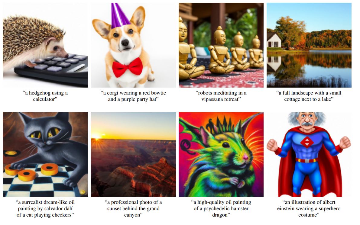
Fig 1. Example outputs of fully-trained GLIDE with image inpaining [1].

Background Architecture

The GLIDE model begins by encoding the text prompt. It first encodes the input text into a sequence of K tokens which are fed into a Transformer model to generate token embeddings. The final token embedding is then fed into an augmented ADM model in place of class embeddings, and the last layer of token embeddings (K feature embeddings) is separately projected to the dimensionality of each attention layer throughout the ADM model, and then concatenated to the attention context at each layer. ADM stands for ablated diffusion model.

The original text prompt is also fed into a smaller transformer model which generates a new set of token embeddings. These embeddings and the 64x64 output of the adapted ADM model are then fed into an upsampling diffusion model with similar residual embedding connections, which will output a 256x256 model generated image.

Transformer Model for Text to Token Encoder

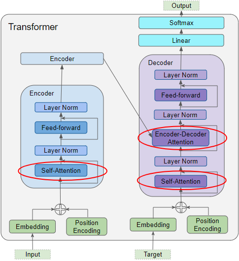
Fig 1. Example of transformer model.

Before inputting out natural language prompt into our transformer model, we must first tokenize it. HuggingFace is by far the market leader for tokenizer applications. Tokenization is the process of encoding a string of text into transformer-readable token ID integers. These token ID integers can be seen as indexes into our total vocabulary list. Once we have this tokenized text input, we then input this into a transformer model in order to generate token embeddings for each input token. These embeddings are a numerical representation of the meaning of the word given both the context and token id. As words can have multiple different meanings in different contexts and may refer to concepts in previous or future parts of the input text, we must develop a sophisticated model to ensure our token embeddings are accurate.

Transformer Models with an attention mechanism through and encoder and decoder rose to fame for this application following the paper Attention is All You Need. Transformers fall under the category of sequence-to-sequence models, in which one sequence, our tokenized input, is translated into a different sequence. We can train our model for token embeddings by masking some inputs and predicting the masked words in the decoder block or through next sentence prediction. The transformer model can be broken into two stages, an encoder and a decoder. After training, we can use the encoder block to generate out token embeddings simply by taking the output of the encoder stack.

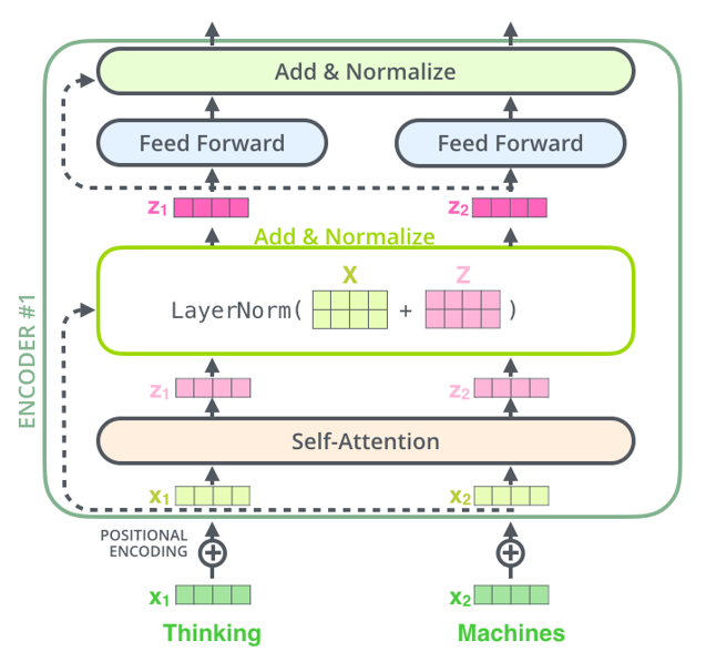
Fig 1. Example of a single encoder module.

The encoder is a stack of encoder modules that sequentially feed into each other to output a final attention and contect vector for the decoder. The orginal tokenized input is first masked, by removing certain words from the input sentence. This masked embedding is put into a self-attention layer which is then normalized and fed through a feed forward neural network with residual connections. Each self-attention layer has three parameters, a query matrix Q, a key matrix K, and a value matrix V. GLIDE uses multi-head attention where each original tokenized input is copied and changed slighlty to include different context or positonal information and fed into our encoder. This can be seens as multiple Q, K, and V vectors that generate seperate output matrices that are concatenated together before being fed into the feed forward layer. This allows the model to learn more nuanced meanings(embeddings) for each word.

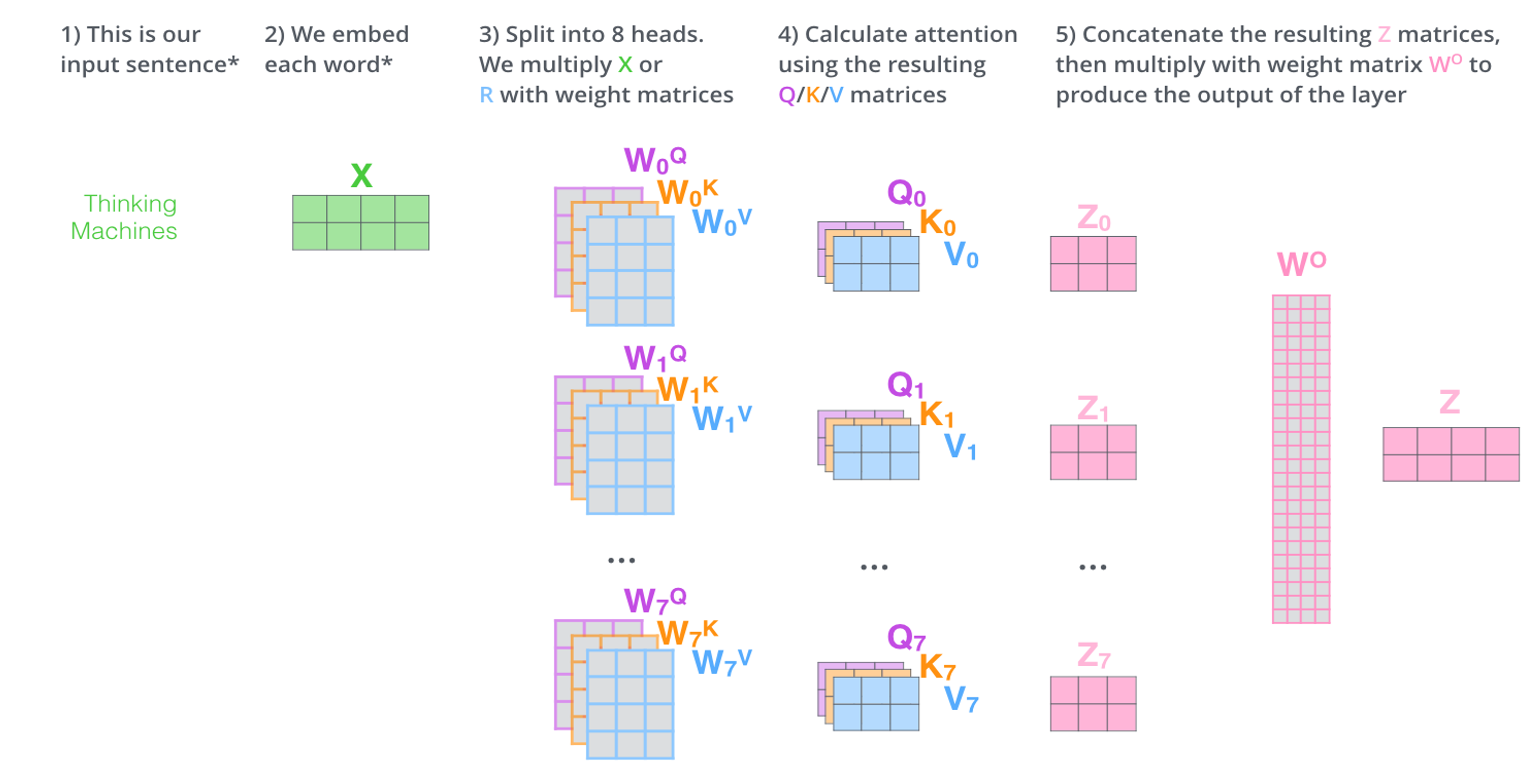
Fig 1. Example of multi-head attention.

Each word will query every other word based on their keys to decide its attention on the words. The query and key vectors for each tokenized input word will then be multiplied and normalized by the square of its size and softmaxed to generate a probability distribution. This is then seen as a score per word of the same length of the input question. This score can be seen has how much that word should pay attention to every other word to inform its embedding meaning. We then multiply this score to the value vector for that word to focus on the words we want to attend to and ignore the others. Our previous input is then added back to this output to emphasize the word to focus more on itself through a residual skip connection.

The initial input into our encoder is our masked tokenized input along with a positional encoding. This positional encoding can be modeled in different ways, and is added to our initial tokenized input to create our transformer input.

After the encoder is finished, a final Key(K) and value(V) matrix is generated and sent to each encode-decode block in the decoder. After training we can throw away the decoder block and keep the endoer block. We then put our use captions that were tokenized into the encoder stack and take the value matrix (NxV) as our token embeddings. The self-attention for the decoder blocks is similar to the encoder but attempts to predict our masked caption. The output of each decoder itteration is fed shifted as input back into the decoder, so it is able to pay attention to all previous outputs when estimating the next word. It has a self-attention layer identical to our encoder blocks, followed by an encoder attention layer, in which it uses a similar process on the K and V matrices from the encoder block to pay attention to the previous caption input.

The Encoder-Decoder Attention is therefore getting a representation of both the target sequence (from the Decoder Self-Attention) and a representation of the input sequence from our encoder final K and V matrices. It produces a representation with the attention scores for each target sequence word that captures the influence of the attention scores from the input sequence. As this passes through all the Decoders in the stack, each Self-Attention and each Encoder-Decoder Attention also add their own attention scores into each word’s representation. We then compare the predicted ouputs for our masked tokenized words to the true ones and reupdate the model. A similar training stage can be done with next sentence prediction rather than a masked tokenized input.

After this is trained, we use the encoder block on out tokenized caption input to extract token embeddings that will be fed into our downsampling then upsampling diffusion models.

For the text encoding Transformer, GLIDE uses 24 residual blocks of width 2048, resulting in roughly 1.2 billion parameters.

Diffusion Model

Diffusion models are a class of likelihood-based models that sample from a Gaussian distribution by reversing a gradual noising process that can be formulated as a Markovian chain. It begins with \(x_T\) and learns to gradually produce less-noisy samples \(x_{T-1},...,x_{1}\) until obtaining \(x_0\). Each reversing of x corresponds to a certain noise level, such that \(x_t\) corresponds to signal \(x_0\) mixed with some noise \(\epsilon\) at a ratio predetermined by t. We assume \(\epsilon\) is drawn from a diagonal Guassian distribution to simplify our equations[5].

So each step of the noising process can be modeled by: \(q(x_t | x_{t-1}) := \mathcal{N}(x_t; \sqrt{α_t}x_{t-1}, (1 -α_t)I )\)

As the magnitude of noise is small at each step but the total noise throughout the Markovian chain is large, \(x_T\) can be approximated by a \(\mathcal{N}(0, I)\).

So each step of the denoising process can be learned as:

\[p_{\theta}(x_{t-1}|x_t) := \mathcal{N}(\mu_{\theta}(x_t), \sum_{\theta}(x_t))\]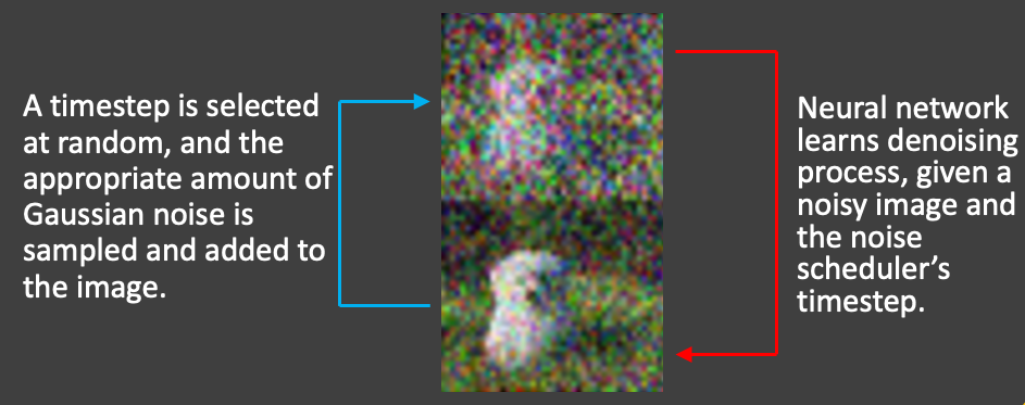

Fig 1. Example Step of Diffusion Model

To train this, we can generate samples \(x_t\) approximated by \(q(x_t | x_0)\) by applying guassian noise to \(x_0\) then train a model \(\epsilon_{\theta}\) to predict the added noise using a surrogate objective. In a basic diffusion model, a simple standard mean-squared error loss can be used. So the outputs and inputs of our convolutional neural network will be seen as inputs and outputs of our diffusion model.

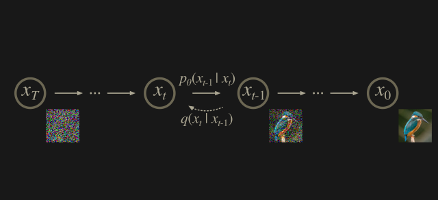
Fig 1. Example of Diffusion Model

GLIDE uses a more efficient version of this where \(\sum_{\theta}\) and \(\mu_{\theta}\) are learned and fixed allowing for much less diffusion steps and a faster training time.

Classifier Free Guidance Loss Functions

Classifier free guidance guides a diffusion model without requiring a seperate classifier model to be trained. Classifier-free guidance allows a model to use its own knowledge for guidance rather than the knowledge of a classification model like CLIP, which generates the most relevant text snippet given an image for label assignment.

In the paper, a CLIP guided diffusion model is compared to a classifier-free diffusion model and finds the classifier-free diffusion model to return mor ephotorealistic results.

For classifier-free guidance with generic text prompts, we replace text captions with an empty sequence at a fixed probability and then guide our prediction towards the true caption (c) using a modified preditiction \(\tilde{\epsilon}\)

\[\tilde{\epsilon_{\theta}}(x_t|c) = \epsilon_{\theta}(x_t| \emptyset) + s \cdot (\epsilon_{\theta}(x_t|c) - \epsilon_{\theta}(x_t|\emptyset))\]

Main Diffusion Model (ADM model architecture with additional text token residual connections)

The ADM architecture builds off of the U-Net CNN architecture[2]. The U-Net model uses a stack of residual layers and downsampling convolutions, followed by a stack of residual layers with upsampling colvolutions, with skip connections connecting the layers with the same spatial size. In addition, they use a global attention layer at the 16×16 resolution with a single head, and add a projection of the timestep embedding into each residual block.

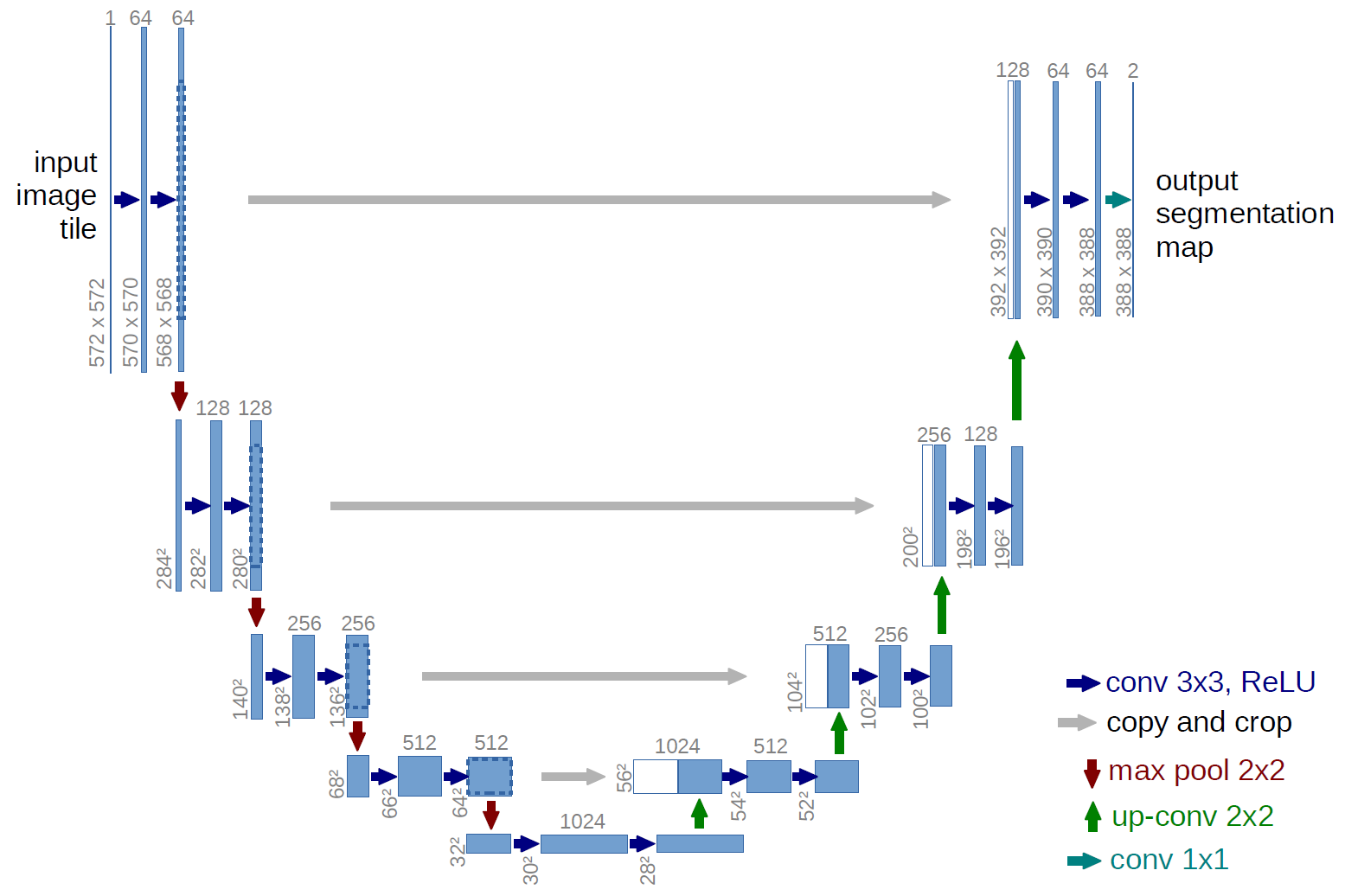
Fig 1. UNet Architecture .

ADM uses this model but creates a new layer called adaptive group normalization (AdaGN), which incorporates the timestep and class embedding into each residual block after a group normalization operation. The layer is defined as \(AdaGN(h, y) = y_sGroupNorm(h)+y_b\), where h is the intermediate activations of the residual block following the first convolution, and \(y = [y_s,y_b]\) comes from a linear projection of the timestep and class embedding.

ADM also incorporates variable width with 2 residual blocks per resolution, multiple heads with 64 channels per head, attention at 32, 16 and 8 resolutions, and BigGAN residual blocks for up and downsampling.

GLIDE adapts this ADM model to use text conditioning information. So, for each noised image \(x_t\) and text caption c, it predicts \(p(x_{t-1}|x_t,c)\)

Additionally, the model width is scaled to 512 channels so it has around 2.3 billion paramters just for the visual part of the model.

Additional Upsampling Diffusion Model

In addition to the augmented ADM model, an additional upsampling diffusion model is trained and increases image size form 64x64 to 256x256. The number of visual base channels used is 384, and a smaller text encoder with 1024 instead of 2048 width is used.

Putting it All Together

So the natural language prompt is first tokenized and encoded. Then the image batch and encodings are fed into the text-adapted ADM model and its low resolution outputs are then fed into the upsampling diffusion model along with a new encoding of the original text input. This will output a 256x256 model generated image.

Training

In the training process, we first trained a text-conditional model. Then the base model is fine-tuned for classifier-free guidance. Model Architecture:

1. ADM 64x64

• model width: 512 channels
• 2.3 billion parameters
• Transformer Model
  • 24 residual blocks of width 2048
  • 1.2 billions
• Iterations: 2.5M
• Batch Size: 2048

1. Upsampling diffusion model:

• model width increases to 384 channels
• text encoder with width 1024
• Transformer Model
  • 24 residual blocks of width 1024
• Iterations: 1.6M
• Batch Size: 512

Dataset

The GLIDE paper simply uses the same dataset used by DALL-E. According to the openai DALL-E github, “The model was trained on publicly available text-image pairs collected from the internet. This data consists partly of Conceptual Captions and a filtered subset of YFCC100M.” Conceptual Captions is a google dataset with 3.3 million images and annotation. YFCC100M is a list of photos and videos. The exact dataset used by both DALL-E and GLIDE has not been released.

Training Process

1. Base Model First step is to encode text into a sequence of K tokens. Then, these tokens are fed into the Transformer model.

2. Upsampling Diffusion model: The upsampling model has the same training process as the base model with some changes in architecture parameters.

3. Classifier-free Guidance Model The training process of the classifier-free guidance model is the same as the base model, except that 20% of the text token sequences are replaced to empty sequence.

Evaluation

In the evaluation process, quantitative metrics, such as Precision/Recall, IS/FID and CLIP score were used. Here we present some simple definitions of each metric:

1. Precision: fraction of relevant images among all generated images.
2. Recall: fraction of relevant images that were generated.
3. Inception Score (IS) The inception score measures 2 things in essence:

1) Image quality: Does the image clearly belong to a certain category?

2) Image diversity: Do the images generated have a large variety?

To evaluate the IS score, we first pass the generated images into a classfier, and we will get a probability distribution of the image belonging to each category.

To test on image quality, the output probability distribution (or conditional probability distribution) of the image should have a low entropy.

To test on image diversity, integrating all the probability distribution of generated images (or marginal probability distribution ) should have a high entropy.

Lastly, we combine the conditional probability and marginal probability using Kullback-Leibler divergence, or KL divergence. The KL divergence is then summed over all images and averaged over all classes.

1. Frechet Inception Distance (FID) Built upon IS, FID aims to measure the photorealism of generated images. It also requires the use of a classifier and feeding the generated images and real images into the classifier. Instead of getting the actual probability distribution, we get rid of the last output layer and use the features of the model, or outputs of the last activation layer. Then we compare the characteristics of the features of generated images and that of the real images. The acutal FID score is the calculated distance between the two feature vectors. A lower FID score means better generated image phtorealism.

2. CLIP CLIP score is defined as \(E[s(f(image)·g(caption))]\) were expectation is taken over the batch of samples, s is the CLIP logit scale, f(image).

Human evaluators were also employed to judge on the photorealistism and caption similarity of the generated images.

Results

From human evaluations, we can see that the classifier-free guidance model outperforms the CLIP-guided model.

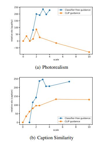
Fig 1. Scores from human evaluations [1].

From quantative metrics, we can see that there is a trade-off between the three pairs of metrics as we increase the guidance scale.

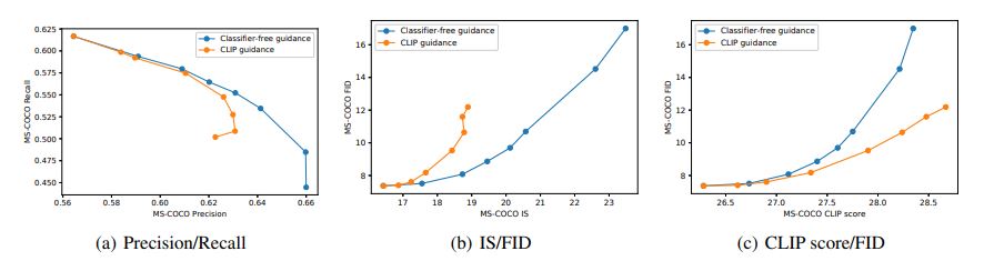
Fig 1. Comparing the diversity-fiedelity trande-off of classifier-free guidance and CLIP guidance [1].

Demo

OpenAI has released a smaller public glide model that filtered out people, faces, and nsfw content.

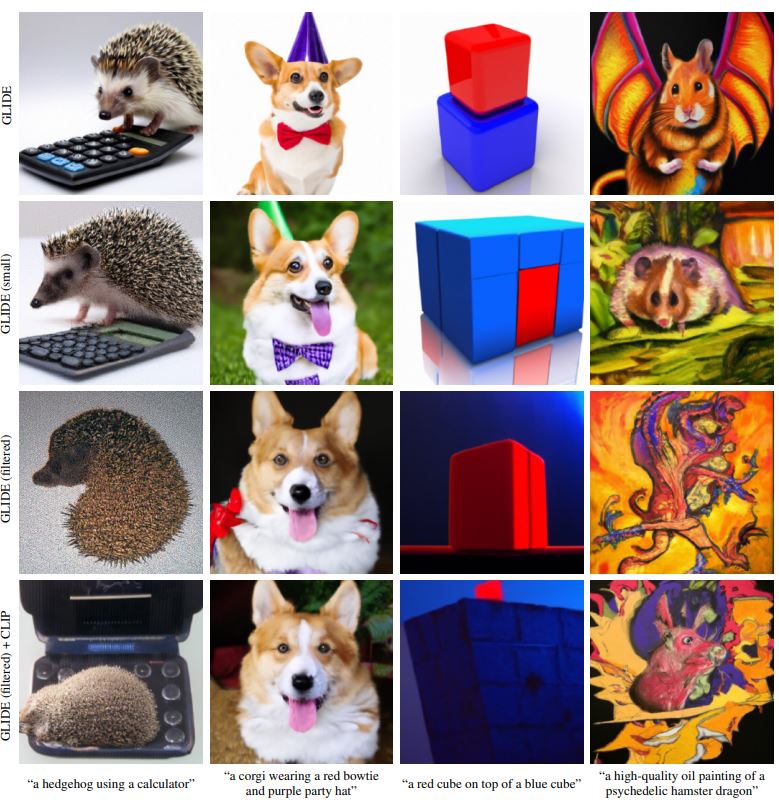
Fig 1. Comparison of full GLIDE model vs Filtered [1].

If you want a quick demo without having to code, github user valhalla has graciously created an interactive website you can try. Interactive Website Link(no coding required, but slower runtime)

OpenAi also released a colab file to play around with their filtered smaller model here.

In addition, we have tried to compare the upsampler model used in the original papaer (augmented ADM model) with another upsampler model, Enhanced Deep Residual Networks (EDSR), using OpenCV. While EDSR has been commonly used to enhance resolution, it is limited to enhance the resolution by up to 4 times. And comparing the results upsampled by ADM and EDSR, we see that the ADM model has achieved better results, as the image is sharp and have high resolution. On the other hand, the EDSR model processes the image faster.

OpenAi also released a colab file to play around with their filtered smaller model here. Based on this colab file, we’ve created a somewhat more beginner-friendly colab file, integrated with the EDSR model. You can try it here. In this demo, we used EDSR model that can enhance resolution by 3 times.

Here is a google colab file we assembled using the OpenAi file and a community recreated version for DALL-E. OpenAi has not released their DALL-E model either for ethical reasons, but the community has tried to reproduce smaller versions of it. The purpose of putting both in our colab file is to easily compare the outputs of filtered GLIDE vs recreated DALL-E. Both GLIDE and DALL-E are the current state of the art zero-shot image generation models, known for their photorealism and diverisity in image generation.

Reference

[1] Nichol, A., Dhariwal, P., Ramesh, A., Shyam, P., Mishkin, P., McGrew, B., Sutskever, I. and Chen, M., 2021. Glide: Towards photorealistic image generation and editing with text-guided diffusion models. arXiv preprint arXiv:2112.10741.

[2] Dhariwal, P. and Nichol, A. Diffusion models beat gans on image synthesis. arXiv:2105.05233, 2021.

[3] Ho, J., Jain, A., and Abbeel, P. Denoising diffusion probabilistic models. arXiv:2006.11239, 2020.

[4] Ho, J. and Salimans, T. Classifier-free diffusion guidance. In NeurIPS 2021 Workshop on Deep Generative Models and Downstream Applications, 2021. URL https:// openreview.net/forum?id=qw8AKxfYbI.

[5] Nichol, A. and Dhariwal, P. Improved denoising diffusion probabilistic models. arXiv:2102.09672, 2021.

[6] Ramesh, A., Pavlov, M., Goh, G., Gray, S., Voss, C., Radford, A., Chen, M., and Sutskever, I. Zero-shot text-toimage generation. arXiv:2102.12092, 2021.

[7] Ashish Vaswani, Noam Shazeer, Niki Parmar, Jakob Uszkoreit, Llion Jones, Aidan N. Gomez, Lukasz Kaiser, and Illia Polosukhin. Attention is all you need. arXiv:1706.03762, 2017.

---