Sheet Music Recognition
Sheet Music Recognition is a difficult task. Zaragoza et al. devised a method for recognizing monophonic scores (one staff). We extend this functionality for piano sheet music with multiple staves (treble and bass). https://github.com/NingWang1729/tf-end-to-end
Main Content
This project was inspired by Zaragoza et al.. We extend the monophonic score reader by parsing grand staves from piano sheet music. Thus, we add a stage in the pipeline to first identify any grand staves before separating them into treble and bass. Each individual staff is then fed into the current pipeline.
An End-to-End Approach to Optical Music Recognition
What is Optical Music Recognition (OMR)?
As its name suggests, OMR is the field of research focused on training computers to automatically read music. Despite its similarities to other processes such as optical character recognition (OCR), OMR is substantially more difficult. Unlike words on a line, the spatial positioning of notes contributes to the overall semantics; for instance, in the treble clef, a note on the bottommost line in a staff is an E, while a note on the line just above it is a G. Furthermore, robust solutions must be able to successfully interpret the same note differently depending on clef, tempo, and a variety of other factors. Other issues include staff lines adding visual noise and hindering note classification, difficulties in finding bars used to delimit staves, and the varying sizes of musical notation (a musical slur may span multiple measures, in contrast to the tiny dots lengthening the duration of a note).
Classical approaches
Traditional methods, not based in deep learning, break down OMR into multiple stages. Among other things, an initial pass will clean up the image by removing staff lines, find the bars that break a stave into measures, and detect the clefs that affect the interpretation of notes in pitches. Next, symbols are isolated and run through a classifier. Finally, the individual components are reassembled and reinterpreted within the overall semantics of the piece.
Unfortunately, such a piecewise approach typically fails to generalize beyond the intended musical formats, due to the manual parameter tuning required for some steps, such as staff-line removal. (Note, for instance, the tuning required in morphological erosion.)
A Deep-Learning Solution
The PrIMuS dataset
Neural networks require large amounts of data upon which to train; to facilitate learning, the authors introduced the Printed Images of Music Staves (PrIMuS) dataset.
In PrIMuS, 87,678 sequences of notes, written upon a single staff, are converted into five different representations, these being
- Plaine and Easie code

Fig 1a. End-to-end neural optical music recognition of monophonic scores. [1].
- Rendered images

Fig 1b. End-to-end neural optical music recognition of monophonic scores. [1].
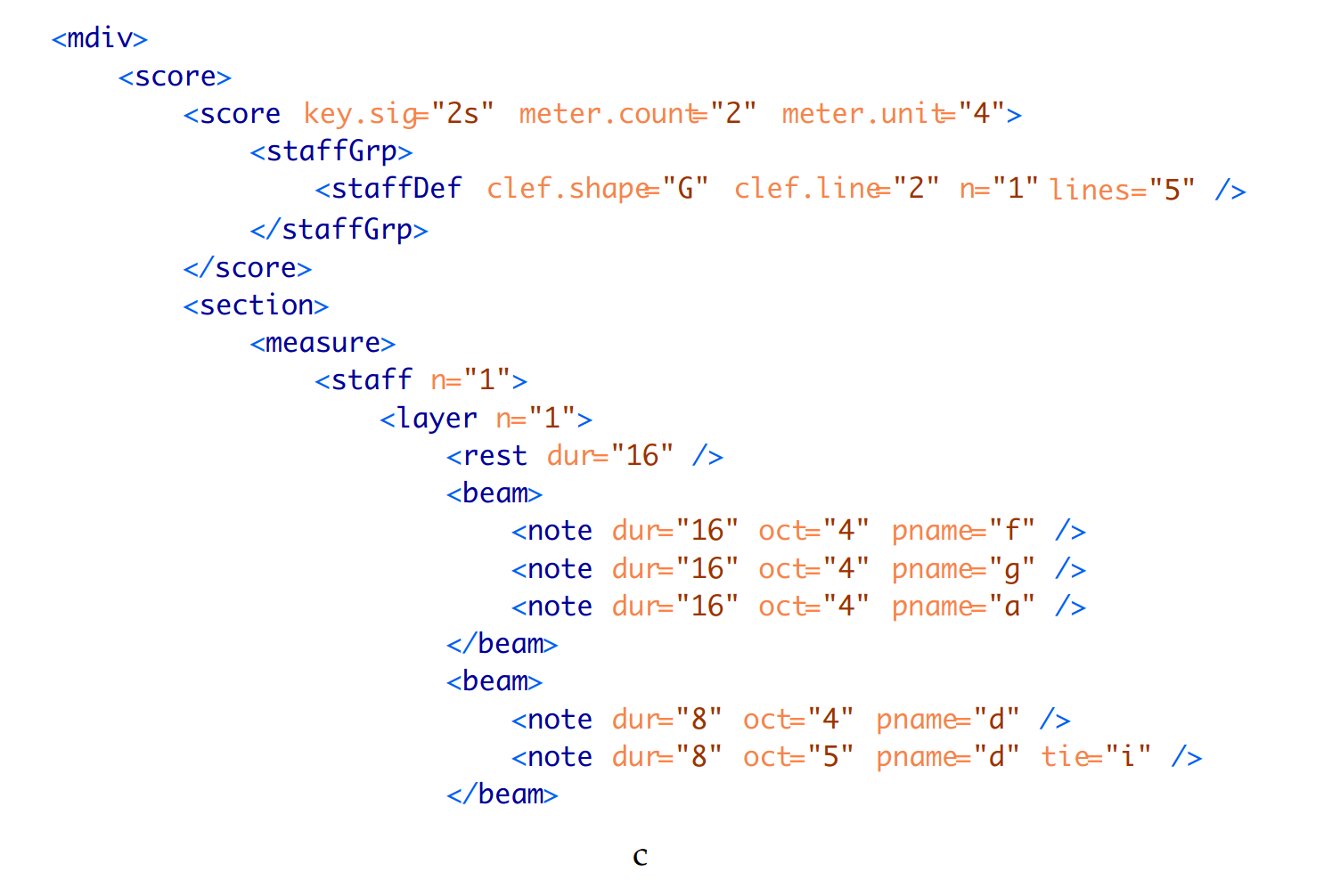
- Music Encoding Initiative format

Fig 1c. End-to-end neural optical music recognition of monophonic scores. [1].
- Semantic encoding

Fig 1d. End-to-end neural optical music recognition of monophonic scores. [1].
- Agnostic encoding

Fig 1e. End-to-end neural optical music recognition of monophonic scores. [1].
Note that in the final setting, many of the rendered images are distorted using GraphicsMagick, so as to emulate pictures taken with a bad camera.
The major accomplishment of PrIMuS, besides its scale and diversity, lies in the distinction between semantic and agnostic encodings. As their names suggest, the semantic encoding includes real musical meaning that the agnostic version lacks. For example, note the two “sharp” symbols in the rendered image above. In the agnostic encoding, these are labelled as
accidental.sharp-L5, accidental.sharp-S3
that is, sharps on “line 5” (the uppermost line) and “space 3” (the third space between two lines). In a real musical context however, these two sharps denote the D-Major key signature, and are appropriately designated
keySignature-DM
in the semantic encoding.
As another example, notes that are linked together (for instance, sixteenth notes) have this visual linkage designated with .beamed in the agnostic representation; in the semantic version, they are correctly labelled .sixteenth.
In essence, the agnostic encoding merely notes the 2D plane positions of musical elements, while the semantic encoding interprets these elements in the context of the greater piece.
A quick primer on CTC networks
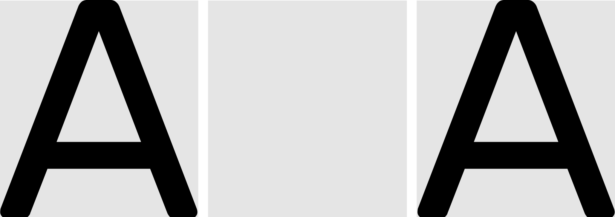
Sequential data usually fails to come in set widths. As an analogy, suppose we had to split a sentence, typed in 20 pt monospace font, into fixed-width letters. This would be easy: all we have to do is box each letter in a rectangle of 20-pt width. Now imagine if we were to use these same boxes to split a second sentence, one written in 25-pt sans-serif. Suddenly, some boxes might contain just a fraction of a character; we would be completely unable to split such a sentence!

How can we fix this? Note that the main problem here is the lack of alignment; a single letter might span two boxes. If we were to independently read each box without the context of the other, we would be unable to make out the greater letter. Thus we need to find some way to span contexts.
Connectionist temporal classification (CTC) accomplishes just this in the context of RNNs. Unlike traditional networks, CTC networks continue predicting the same token when the current context is not yet finished; for instance, in our example above, given

, a network might learn to predict AAA, because the network correctly recognizes that the latter two boxes still span the A.
Note that with this current system, we are unable to distinguish whether AAA corresponds to A, AA, or a true AAA. With CTC, the solution is to add a special “blank” character - that delimits tokens. Therefore given

, a CTC network might predict A-A.
To formalize the above, a CTC network uses an RNN to map from a \(T\)-length sequence \(\textbf{x}\) to a \(T\)-length target sequence \(\textbf{z}\). Each element \(x_i \in \mathcal{X}\), the \(i\)th element of \(\textbf{x}\), is an \(m\)-dimensional real-valued vector. Given a finite alphabet \(\Sigma\), consisting of all possible token labels, \(z_i \in \Sigma^* = \Sigma \cup \{\text{blank}\}\). Each output unit in the network calculates the probability \(y_k^t\) of observing the corresponding label at time \(t\); as it is assumed all such probabilities are independent among the \(T\) indices, then given an output sequence \(\pi\), the probability \(p\) of getting output sequence \(\pi\) given input sequence \(\textbf{x}\) is
\[p(\pi \mid \textbf{x}) = \prod_{t=1}^T y_{\pi_t}^t.\]All blanks and duplicates are removed after final processing, so sequences such as --lll-m--aa-o and lm-ao both map to lmao. Therefore the probability of getting a final labelling \(\textbf{l}\) is
The predicted sequence is that with the highest probability, or
\[\arg \max_{\textbf{l} \in L^{\leq T}} p(\textbf{l} \mid \textbf{x}).\]The deep-learning approach
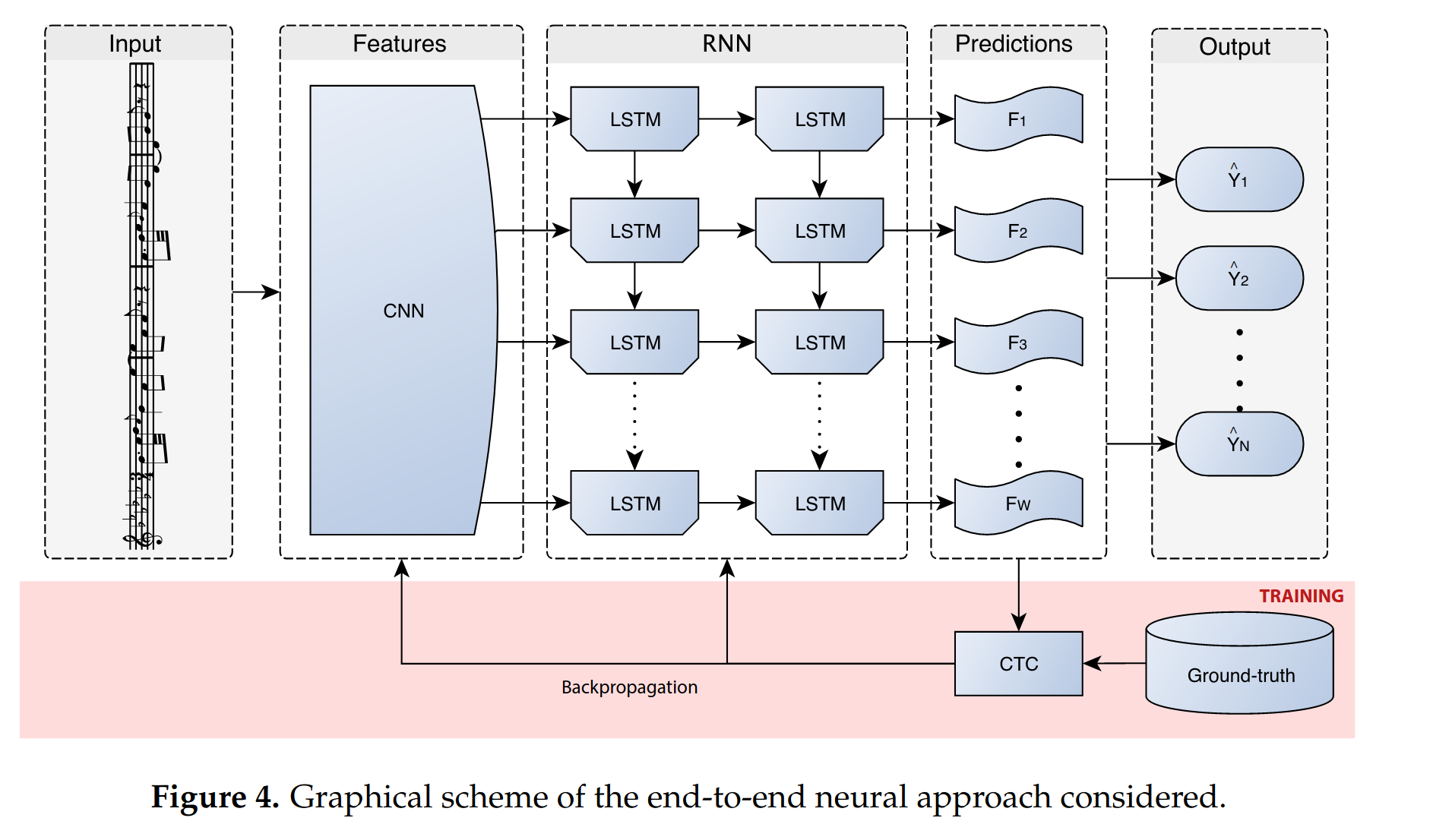
Since music is a prime example of sequential data without fixed widths, the authors have chosen to create a Convolutional Recurrent Neural Network (CRNN) leveraging CTC loss. To simplify the process, only single staffs are run through the network (so, for instance, the network cannot simultaneously process the two staffs—one for each hand—of a piano piece).
The model structure is as follows:

Fig 4. End-to-end neural optical music recognition of monophonic scores. [1].
Specifically, we have
| Input (\(128 \times W \times 1\)) |
|---|
| Convolutional Block |
| Conv(\(32, 3 \times 3\)), MaxPool(\(2 \times 2\)) |
| Conv(\(64, 3 \times 3\)), MaxPool(\(2 \times 2\)) |
| Conv(\(128, 3 \times 3\)), MaxPool(\(2 \times 2\)) |
| Conv(\(256, 3 \times 3\)), MaxPool(\(2 \times 2\)) |
| Recurrent Block |
| Bidirectional LSTM(\(256\)) |
| Bidirectional LSTM(\(256\)) |
| Linear(\(|\Sigma| + 1\)) |
| Softmax |
, where the input is given in \((h, w, c)\) format. Batch normalization is used for every convolutional layer, and the outputs of said layers are passed through a standard ReLU. Note that the linear layer has \(|\Sigma| + 1\) output units because of the extra blank label needed with CTC. Bidirectional LSTMs are used because later information about notes can help inform previous frames.
In training, mini-batches of 16 samples and the Adadelta learning rate optimizer were used. While there are better ways to decode the final sequence (i.e. beam search), a simple greedy decoding is used.
Baseline results
The paper defines two error metrics, the sequence error rate, the percentage of predicted sequences with at least one error; and the symbol error rate, the average edit distance between the predicted and ground truth sequence. The results are as follows:
| Agnostic | Semantic | |
|---|---|---|
| Sequence error rate (%) | 17.9 | 12.5 |
| Symbol error rate (%) | 1.0 | 0.8 |
Notably, the model performs much better on the semantic representation, likely due to its closer ties to the actual musical notation.
Improving Upon the Paper
We extend the functionality of this paper from single staff monophonic scores to full piano sheet music with two staves and monophonic lines in each staff. For this purpose, we use Johann Sebastian Bach’s Two Part Inventions for our training, validation, and test data. The Two Part Inventions are an ideal material to use for this extension as each line contains a single monophonic score. Thus, our task becomes an object detection task to identify grand staves from the full page of sheet music and pass each staff from the grand staff (treble and bass) to the OMR script.
For object detection, rather than reinventing the wheel, we used YOLOv5 to detect the grand staffs. YOLOv5 uses a model backbone, model neck, and model head in its structure. The model backbone extracts the features using Cross Stage Partial Networks. The model neck uses PANet for obtaining feature pyramids. The model head finally predicts the object locations from the image. Training on YOLOv5 requires both input images as well as files with the labels for each object in each image.
Training data was bootstrapped from the first 9 inventions. These 9 inventions were each two pages of sheet music, with 5 or 6 grand staves per page. These staves were croppped and randomly sampled into 5 staves per page training examples and 6 staves per page training examples. 2500 examples were generated using bootstrap for 5 and 6 pages each respectively, for 5000 total training examples. These grand staff locations were manually labeled, and the new locations were passed on to the full sheet music examples. We used the pretrained weights yolov5l.pt for our training.
The 10th through 12th inventions were used to validate the grand staff identification. YOLOv5 was able to correctly identify each grand staff, for both the 5 and 6 grand staves per page examples. Finally, the 13th through 15th inventions were reserved as the sample space for the test set for both the object detection as well as the actual OMR. These images with labels were then used to crop the grand staves, which were split in half into treble and bass clefs. These single staves were then passed into the OMR script for semantic and agnostic predictions.
Results
The grand staff detection had perfect accuracy. However, the results for the OMR part of the pipeline are more nuanced; notably, the agnostic encoding proves better than the semantic encoding.
First, we examine the semantic model for the treble clef of the first line of Bach’s Invention no. 13 in A minor. Here we have a very interesting phenomenon. In piano, there are two clefs used: treble (G clef) and bass (F clef). However, there are other clefs used in other forms of music. Here, our model incorrectly predicted the clef to be the soprano clef, one of the C-clefs, when in reality it should be a treble clef. Thus, if strictly interpreting this as treble clef, we would have 0% accuracy for the notes. However, reading the soprano clef, we would have 95% accuracy for the notes, though one note was double counted. As for the non-note markings, the barlines are all predicted except for the first one. However, the slurs have been misread as ties. While the time signature was correctly read as C, for common time, the key signature was incorrectly interpreted as F major instead of A minor. The rests were correctly identified. On the other hand, the agnostic model performed superbly. Every single note was correctly identified with the correct line and direction of beams. The sharp was also identified, which was missed by the semantic version. In the key of A minor, this is the crucial leading tone of G-sharp for the harmonic minor. The model also identified the end of the slur, which was misread as a tie by the semantic model. However, the clef was still misread as a soprano C-clef rather than treble clef.
Next, we examine the semantic model for the bass clef for the same portion of Bach’s Invention no 13. in A minor. Here, we see the bass clef misidentified as treble clef. As seen previously, if interpreting as treble clef, we have a high accuracy for notes of 91%, with the only errors being two E#’s being read as C# for some reason. The barlines were correctly identified but the slurs were again read as ties. The key signature was read as Bb major, which is strange as there are no flats in the key signature, but the time signature was accurately predicted as common time. For the agnostic model, we had better results. Here, we have 91% accuracy for the notes, with the first note being misread as a flat, and the third node being read in the wrong space. Interestingly, the second slur start was correctly predicted, and the second slur end was correctly predicted, although the first slur was missed. The clef was not found, but the first bar line was found instead.
Overall conclusions
The YOLO model was able to correctly identify grand staffs. However, the following OMR model was not so lucky. It misread the clefs for the semantic encoding, which meant the result would be transposed to the wrong key. However, the agnostic model showed that out of context, it could read what the music has written. These imperfections may largely be due to the fact that the OMR was trained on monophonic scores and was therefore not used to reading piano scores. The training data contained other staves than treble and bass, which made a large amount of the training data irrelevant to the piano music. The other test examples shared similar patterns as described for these two staves (misidentified clefs but largely correct notes when transposed). Due to the absurdly high level of musical understanding required to parse these results and overwhelming intensity of transposing between clefs not usually familiar to pianists, no further test cases were used for these detailed evaluations.
Demonstration:
https://colab.research.google.com/drive/1Qgn8U2iB3LoddkgIT2nSDSJwal-ECuOs
https://youtu.be/uD7JU61pI_U
Reference
[1] Calvo-Zaragoza, J., Rizo, D.: End-to-end neural optical music recognition of monophonic scores. Appl. Sci. 8(4), 606 (2018)
[2] Calvo-Zaragoza, J., Rizo, D.: Camera-PrIMuS: neural end-to-end optical music recognition on realistic monophonic scores. In: Proceedings of the 19th International Society for Music Information Retrieval Conference, ISMIR 2018, Paris, France, 23–27 September 2018, pp. 248–255 (2018)
[3] Alfaro-Contreras M., Calvo-Zaragoza J., Iñesta J.M. (2019) Approaching End-to-End Optical Music Recognition for Homophonic Scores. In: Morales A., Fierrez J., Sánchez J., Ribeiro B. (eds) Pattern Recognition and Image Analysis. IbPRIA 2019. Lecture Notes in Computer Science, vol 11868. Springer, Cham.
[4] Graves, Alex & Fernández, Santiago & Gomez, Faustino & Schmidhuber, Jürgen. (2006). Connectionist temporal classification: Labelling unsegmented sequence data with recurrent neural ‘networks. ICML 2006 - Proceedings of the 23rd International Conference on Machine Learning. 2006. 369-376. 10.1145/1143844.1143891.