Medical Image Segmentation
The use of deep learning methods in medical image analysis has contributed to the rise of new fast and reliable techniques for the diagnosis, evaluation, and quantification of human diseases. We will study and discuss various robust deep learning frameworks used in medical image segmentation, such as PDV-Net and ResUNet++. Furthermore, we will implement our own neural network to explore and demonstrate the capabilities of deep learning in this medical field.
- Main Content
- Progressive Dense V-Network
- ResUNet++
- Demo
- References
- [6] Zimmermann-Fraedrich et al., “Right-sided location not associated with missed colorectal adenomas in an individual-level reanalysis of tandem colonoscopy studies,” Gastroenterology, vol. 157, no. 3, pp. 660–671, 2019.
Main Content
Our team explores the applications of CV in healthcare; specifically, notable state-of-the-art medical image segmentation methods. Areas of interest include biomimetic frameworks for human neuromuscular and visuomotor control, segmentation of mitochondria, and segmentation of healthy and pathological lung lobes.
Example
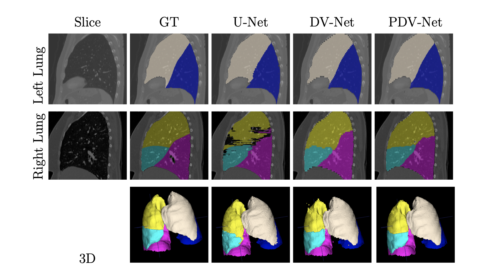
Fig 1. Automatic Segmentation of Pulmonary Lobes [1].
V-Net
Convolutional neural networks have been popular for solving problems in medical image analysis. Most of the developed image segmentation approaches only operate on 2D images. However, medical imaging often consists of 3D volumes, which gives opportunity to the development of CNNs in 3D image segmentation. In their paper V-Net: Fully Convolutional Neural Networks for Volumetric Medical Image Segmentation, Milletari et al propose the V-Net: a volumetric, fully convolutional neural network trained on 3D MRI scans of the prostate to predict segmentation for the entire volume.
Importance: “Segmentation is a highly relevant task in medical image analysis. Automatic delineation of organs and structures of interest is often necessary to perform tasks such as visual augmentation [10], computer assisted diagnosis [12], interventions [20] and extraction of quantitative indices from images [1]. In particular, since diagnostic and interventional imagery often consists of 3D images, being able to perform volumetric segmentations by taking into account the whole volume content at once, has a particular relevance.”
Unlike prior approaches for processing 3D image inputs slice-wise (with 2D convolutions on each slice), the proposed model uses volumetric (3D) convolutions. The following figure is a schematic representation of the V-Net model. The left side of the figure depicts a compression path, while the right side depicts a decompression path to the original signal size. Each intermediate “stage” consists of 2-3 convolutional layers. Moreover, the input of each stage is “(a) used in the convolutional layers and processed through the non-linearities and (b) added to the output of the last convolutional layer of that stage in order to enable learning a residual function”. The design of this neural network ensures a runtime much faster than similar networks that do not learn residual functions.
Along the compression path, the data resolution is reduced with convolution kernels of dimensions 2 × 2 × 2 applied at stride 2, effectively halving the size of feature maps at each stage. Additionally, the number of feature channels and in turn number of feature maps doubles at each compression stage. Conversely, the decompression stages apply de-convolutions to increase the data size again, while also accounting for previously extracted features from the left path. The final predictions, after a softmax layer, comprises two volumes outputting the probability of each voxel to belonging to foreground and to background.
The objective function used by the V-Net architecture considers the dice coefficient, a quantity ranging from 0 to 1. The dice coefficient between two binary volumes is defined as
\[D = \dfrac{2 \sum_{i}^{N} p_i g_i}{ \sum_{i}^{N} p_i^{2} + \sum_{i}^{N} g_i^{2} }\]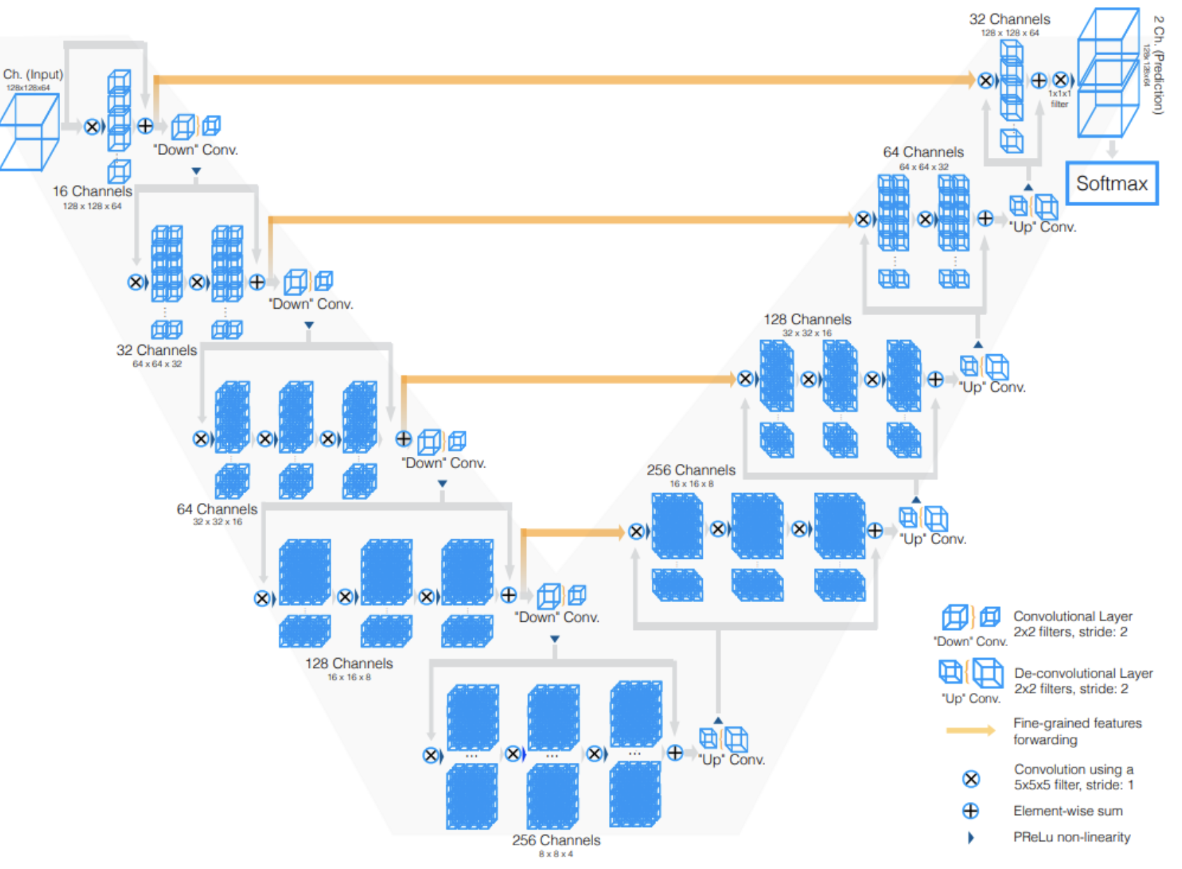 Fig 2. V-Net Architecture [1].
Code Implementation
The traditional V-Net is a fully convolutional deep neural network operating on 3D volumes of medical scans; it consists of an “encoder” network followed by a “decoder” network with outputs forwarded from the encoder blocks to decoder blocks.
There is an initial block which performs 5x5x5 convolution on the input, increases the number of channels from 1 to 16, performs batch normalization and PReLU, and adds this result to the original input.
class InBlock(nn.Module):
    def __init__(self, c_in, c_out):
        super().__init__()
        self.c_out = c_out
        self.conv = nn.Conv3d(c_in, c_out, kernel_size=5, padding=2)
        self.batchnorm = nn.BatchNorm3d(c_out)
        self.prelu = nn.PReLU(c_out)

    def forward(self, x):
        out = self.conv(x)
        out = self.batchnorm(out)
        out = self.prelu(out)
        x_repeat = torch.cat([x]*self.c_out, dim=1)
        out = out + x_repeat
        return self.prelu(out)
Encoder network blocks (“down blocks”) are comprised of a “downsampling” convolution of kernel size 2, stride 2, followed by multiple convolutional layers of kernel size 5, padding 2. The intermediate tensors also undergo batch normalization and PReLU activation.
class DownBlock(nn.Module):
    def __init__(self, c_in, c_out, num_convs, use_batchnorm=True, use_dropout=False):
        super().__init__()
        self.num_convs = num_convs
        self.down_conv = nn.Conv3d(c_in, c_out, kernel_size=2, stride=2)
        self.prelu = nn.PReLU(c_out)
        self.conv = nn.Conv3d(c_out, c_out, kernel_size=5, padding=2)
        if use_batchnorm:
            self.batchnorm = nn.BatchNorm3d(c_out)
        else:
            self.batchnorm = nn.Identity()
        if use_dropout:
            self.dropout = nn.Dropout3d()
        else:
            self.dropout = nn.Identity()

    def forward(self, x):
        out = self.down_conv(x)
        out = self.batchnorm(out)
        out = self.prelu(out)
        out = self.dropout(out)
        out_copy = torch.clone(out)
        for _ in range(self.num_convs):
            out = self.conv(out)
            out = self.batchnorm(out)
            out = self.prelu(out)
        out = out + out_copy
        return self.prelu(out)
Through each encoder block, the number of channels is doubled.
Decoder network blocks (“up blocks”) are comprised of a “upsampling” transposed convolution of kernel size 2, stride 2, followed by multiple convolutional layers of kernel size 5, padding 2. The intermediate tensors also undergo batch normalization and PReLU activation.
class UpBlock(nn.Module):
    def __init__(self, c_in, c_out, num_convs, use_batchnorm=True):
        super().__init__()
        self.num_convs = num_convs
        self.up_conv = nn.ConvTranspose3d(c_in, c_out // 2, kernel_size=2, stride=2)
        self.prelu_in = nn.PReLU(c_out // 2)
        self.conv = nn.Conv3d(c_out, c_out, kernel_size=5, padding=2)
        self.prelu = nn.PReLU(c_out)
        if use_batchnorm:
            self.up_batchnorm = nn.BatchNorm3d(c_out // 2)
            self.batchnorm = nn.BatchNorm3d(c_out)
        else:
            self.up_batchnorm = nn.Identity()
            self.batchnorm = nn.Identity()

    def forward(self, x, x_forwarded):
        out = self.up_conv(x)
        out = self.up_batchnorm(out)
        out = self.prelu_in(out)
        out = torch.cat((out, x_forwarded), dim=1)
        out_copy = torch.clone(out)
        for _ in range(self.num_convs):
            out = self.conv(out)
            out = self.batchnorm(out)
            out = self.prelu(out)
        out = out + out_copy
        return self.prelu(out)
Through each decoder block, the number of channels is halved.
Lastly, there is a final block consisting of two 1x1x1 convolutions with stride 1, followed by a softmax to output the final result. The output has 2 channels, one predicting the foreground and the other predicting the background at pixel level.
class OutBlock(nn.Module):
    def __init__(self, c_in, c_out):
        super().__init__()
        self.batchnorm = nn.BatchNorm3d(c_out)
        self.prelu = nn.PReLU(c_out)
        self.softmax = F.softmax
        self.conv = nn.Conv3d(c_in, c_out, kernel_size=1)
        self.conv2 = nn.Conv3d(2, 2, kernel_size=1)

    def forward(self, x):
        out = self.conv(x)
        out = self.batchnorm(out)
        out = self.prelu(out)
        out = self.conv2(out)
        out = self.softmax(out)
        return out
The V-Net implementation has the following code, using the block modules defined above:
class VNet(nn.Module):
    def __init__(self):
        super().__init__()
        self.p_in = InBlock(1, 16)
        self.down1 = DownBlock(16, 32, 2)
        self.down2 = DownBlock(32, 64, 3)
        self.down3 = DownBlock(64, 128, 3)
        self.down4 = DownBlock(128, 256, 3)
        self.up1 = UpBlock(256, 256, 3)
        self.up2 = UpBlock(256, 128, 3)
        self.up3 = UpBlock(128, 64, 3)
        self.up4 = UpBlock(64, 32, 2)
        self.p_out = OutBlock(32, 2)

    def forward(self, x):
        out_in = self.p_in(x)
        out_down1 = self.down1(out_in)
        out_down2 = self.down2(out_down1)
        out_down3 = self.down3(out_down2)
        out_down4 = self.down4(out_down3)
        out = self.up1(out_down4, out_down3)
        out = self.up2(out, out_down2)
        out = self.up3(out, out_down1)
        out = self.up4(out, out_in)
        out = self.p_out(out)
        return out
Next, we compared models of different depths. The “depth” refers to the number of encoding / decoding stages – i.e., a depth 4 V-Net has 4 encoder blocoks followed by 4 decoder blocks (the common size for image segmentation architectures). To evaluate the impact of depth on the architecture’s effectiveness, we trained two models: 1. (standard model) V-Net of depth 4: - 4 encoder stages followed by 4 decoder stages - flow of # channels: 1 -> 16 -> 32 -> 64 -> 128 -> 256 -> 128 -> 64 -> 32 -> 2 2. V-Net of depth 3: - 3 encoder stages followed by 3 decoder stages - flow of # channels: 1 -> 16 -> 32 -> 64 -> 128 -> 64 -> 32 -> 2
Both models were trained for 20 epochs with Adam optimizer with learning rate 0.01 and weight decay 1e-6. Example results are depicted below. (Columns are in order of original scan, ground truth segmentation, depth 4 model prediction, depth 3 model prediction.)
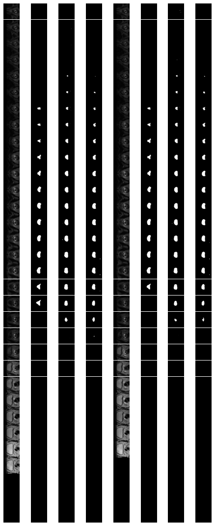 Fig 2. VNet Depth Comparision
We also compared depth 4 V-Net models with different channel flows: 1. (standard model) number of channels: 1 -> 16 -> 32 -> 64 -> 128 -> 256 -> 128 -> 64 -> 32 -> 2 2. number of channels: 1 -> 8 -> 16 -> 32 -> 64 -> 128 -> 64 -> 32 -> 16 -> 2 3. number of channels: 1 -> 4 -> 8 -> 16 -> 32 -> 64 -> 32 -> 16 -> 8 -> 2
Again, all three models were trained for 20 epochs with Adam optimizer with learning rate 0.01 and weight decay 1e-6. Example results of this comparison are depicted below. (Columns are in order of original scan, ground truth segmentation, model #1 prediction, model #2 prediction, model #3 prediction.)
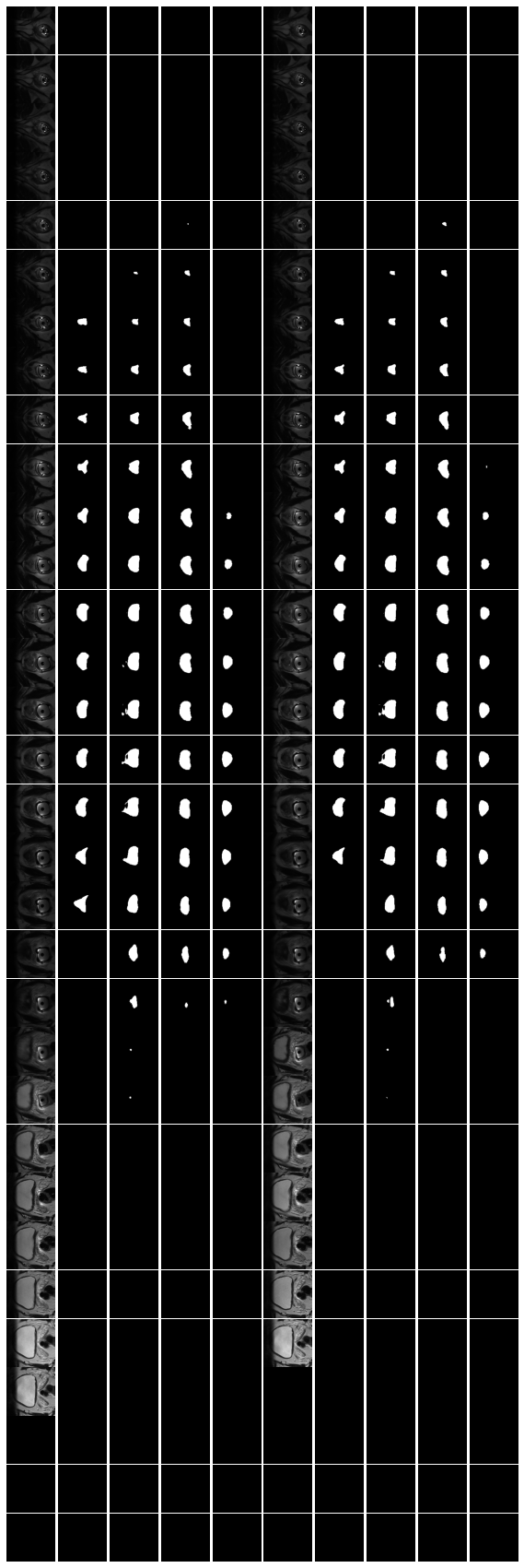 Fig 3. VNet Channel Comparision
Progressive Dense V-Network
Motivation
In the medical imaging analysis field, fast and reliable segmentation of lung lobes is important for diagnosis, assessment, and quantification of pulmonary diseases. Existing techniques for segmentation have been slow and not fully automated. To address the lack of an adequate imaging system, this paper proposes a new approach for lung lobe segmentation: a progessive dense V-network (PDV-Net) that is robust, fast, and fully automated. Some challenges to develop efficient automated system to identify lung fissures are as follows:
- Fissures are usually incomplete, not extending to the lobar boundaries.
- Visual characteristics of lobar boundaries vary in the presence of pathologies.
- Other fissures may be misinterpreted as the major or minor fissures that separate the lung lobes. The authors discuss prior deep learning developments in the medical image segmentation field, such as the dense V-network and progressive holistically nested networks. These approaches were slow and generally low in performance for pathological cases. The proposed PDV-Net model mitigates these limitations, and uses the following architecture.
Architecture
The input is down-sampled and concatenated with a convolution of the input, where the convolution has 24 kernels of size 5 x 5 x 5 and stride 2. This is passed onto three dense feature blocks: one block with 5 and two blocks with 10 densely connected convolutional layers. The three dense blocks have growth rates 4, 6, and 8, respectively. All of their convolutional layers have 3 x 3 x 3 kernels and are followed by batch normalization and PReLU.
The dense block outputs are consecutively forwarded in low and high resolution passes via compression and skip connections, which enables the generation of feature maps at three different resolutions. The outputs of the skip connections of the second and third dense feature blocks are decompressed to match the first skip connection’s output size. The merged feature maps from the skip connections are passed to a convolutional layer followed by a softmax, to output the final probability maps. This proposed architecture progressively improves the outputs from previous pathways to output the final segmentation result. Similar to the V-Net solution, it utilizes a dice-based loss function for model training. To train the network, the training volumes are first normalized and rescaled to 512 x 512 x 64. Spatial batch normalization and dropout are incorporated for regularization. Moreover, the authors use the Adam optimizer with learning rate 0.01 and weight decay 10-7.
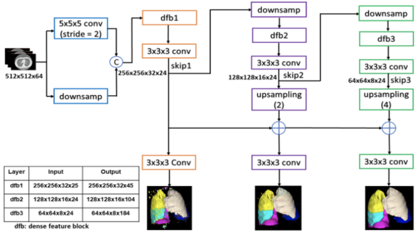 Fig 4. Architecture for Progressive Dense V-Network [2].
Results
Using the dice score for comparison, the authors find that the PDV-Net significantly outperforms the 2D U-Net model and the 3D dense V-Net model. Further investigations show that the PDV-Net is robust against the reconstruction kernel parameters, different CT scan vendors, and presence of lung pathologies. Additionally, the model takes approximately 2 seconds segment lung robes from a single CT scan, which is faster than all prior solutions at the time of its proposal.
ResUNet++
Motivation
Colonoscopy plays an important part of colorectal cancer detection. However, existing examination methods are hampered by high overall miss rate and many abnormalities. According to recent studies, polyps smaller than 10 mm, sessile, and flat polyps [5] are shown to most often be missed [6]. Thus, developing a computer-guided diagnosis system for polyp segmentation can assist in monitoring and increasing the diagnostic ability by increasing the accuracy, precision, and reducing manual intervention [2].
Architecture
As its name suggests, ResUNet++ is derived from the backbone architecture ResUNet, an encoder-decoder network based on U-Net. ResUNet also employs and utilizes the properties of residual blocks, squeeze and excite blocks, spatial pyramid poolings (ASPP), and attention blocks. ResUNet++ improves ResUNet by introducing:
- the sequence of squeeze and excitation block to the encoder part of the network
- the ASPP block at the bridge and decoder
- the attention block at the decoder
The overall ResUNet architecture could be described as one stem block followed by three encoder blocks then three decoder blocks, all of which (the blocks) use the standard residual learning approach. The output of the last decoder block is passed through the ASPP, then a 1x1 convolution and a sigmoid activation function. Note that all convolution layers (except the output layer) are batch normalized and activated by ReLU activation function.
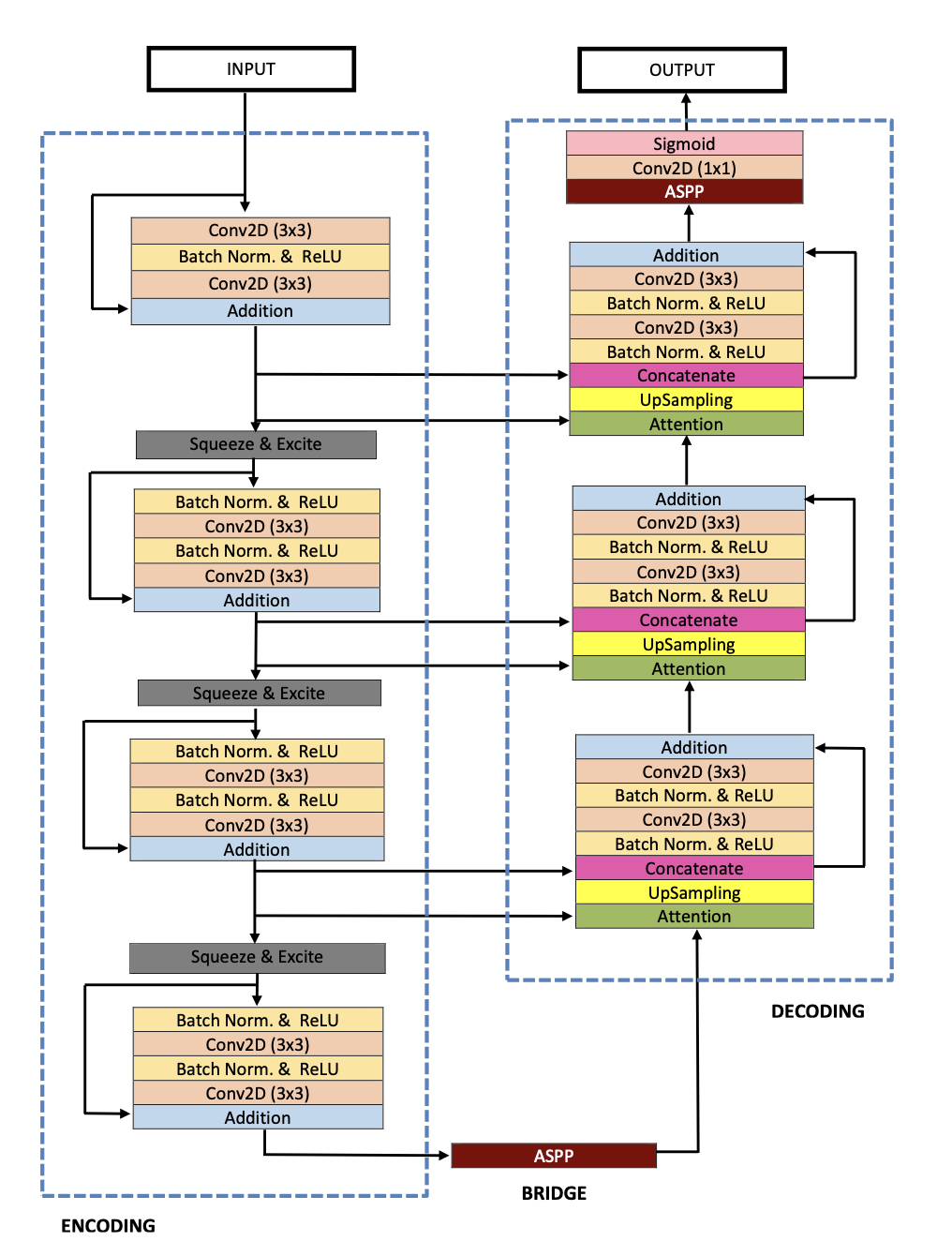 Fig 5. Architecture for ResUNet++ [3].
Architecture Blocks and Code Implementation
Each block of the architecture plays an important role in the performance of the model. Below we describe the functions of each block and how they enable model performance.
- Residual Block: enables network to expand depth without running into problems with exploding/ vanishing gradients during backpropogation. Residual-based networks simplifies the objective of optimization to learning the identity function; thus providing skip connections.
class RESBLOCK(nn.Module):
  def __init__(self, CIN, COUT, STRIDES=1):
    super(RESBLOCK, self).__init__()
    # N, C, H, W
    self.convn3 = Conv2dSame(CIN, COUT, (3,3), stride=STRIDES)
    self.convn1 = Conv2dSame(CIN, COUT, (1,1), stride=STRIDES)
    self.conv1 = nn.Conv2d(COUT, COUT, (3,3), padding="same")
    self.norm1 = nn.BatchNorm2d(CIN)
    self.norm2 = nn.BatchNorm2d(COUT)
    self.act = nn.ReLU()
    self.sqzext = SQUEEZEXCITE(COUT)

  def forward(self, x):
    out = self.norm1(x)
    out = self.act(out)
    out = self.convn3(out)

    out = self.norm2(out)
    out = self.act(out)
    out = self.conv1(out)

    x = self.convn1(x)
    x = self.norm2(x)

    out = out + x
    out = self.sqzext(out)

    return out
- Squeeze and Excitation (SE) Block: enables network to perform dynamics channel-wise feature recalibration. To model interdependencies between the channels, SE “squeezes” on the feature maps using global average pooling, the output of which is fed into sigmoid to add non-linearity in capturing the channel-wise dependencies. The feature map of the convolution block is then weighted acrrodingly (“excitation”).
class SQUEEZEXCITE(nn.Module):
    def __init__(self, CIN, RATIO=2):
        super(SQUEEZEXCITE, self).__init__()
        reduction = CIN // RATIO
        self.ration = RATIO
        self.fc1 = nn.Linear(CIN, reduction, bias=True)
        self.fc2 = nn.Linear(reduction, CIN, bias=True)
        self.relu = nn.ReLU()
        self.sigmoid = nn.Sigmoid()

    def forward(self, x):
        N, C, H, W = x.size()
        # global avg pooling
        s = x.view(N, C, -1).mean(dim=2)
        # channel excitation
        out = self.relu(self.fc1(s))
        out = self.sigmoid(self.fc2(out))

        a, b = s.size()
        output_tensor = torch.mul(x, out.view(a, b, 1, 1))
        return output_tensor
- Atrous Spatial Pyramid Pooling: captures the contextual information at different scales by probing a given image/ feature with multile filters that have complementary effective fields of view. This is used as a bridge between the encoder and edcoder to learn the multi-scale information between the encoder and decoder.
class ASPP(nn.Module):
  def __init__(self, CIN, COUT, SCALE=1):
    super(ASPP, self).__init__()
    self.conv1 = nn.Conv2d(CIN, COUT, (3,3), padding="same", dilation=(6*SCALE, 6*SCALE))
    self.conv2 = nn.Conv2d(CIN, COUT, (1,1), padding="same", dilation=(12*SCALE, 12*SCALE))
    self.conv3 = nn.Conv2d(CIN, COUT, (3,3), padding="same", dilation=(18*SCALE, 18*SCALE))
    self.conv4 = nn.Conv2d(CIN, COUT, (3, 3), padding="same")
    self.conv5 = nn.Conv2d(COUT, COUT, (1, 1), padding="same")
    self.norm = nn.BatchNorm2d(COUT)

  def forward(self, x):
    out1 = self.conv1(x)
    out1 = self.norm(out1)

    out2 = self.conv2(x)
    out2 = self.norm(out2)

    out3 = self.conv3(x)
    out3 = self.norm(out3)

    out4 = self.conv4(x)
    out4 = self.norm(out4)

    out = out1 + out2 + out3 + out4
    out = self.conv5(out)

    return out
- Attention Units: gives importance to the subset of the network to highlight the most relevant information by allowing the model to visualize the feautres importance at different scales and positions. This is thought to be an improvement over average and max pooling base-line.
class ATTENTION(nn.Module):
  def __init__(self, CIN1, CIN2, COUT, SCALE=1):
    super(ATTENTION, self).__init__()
    self.conv1 = nn.Conv2d(CIN1, COUT, (3, 3), padding="same")
    self.conv2 = nn.Conv2d(CIN2, COUT, (3,3), padding="same")
    self.norm1 = nn.BatchNorm2d(CIN1)
    self.norm2 = nn.BatchNorm2d(CIN2)
    self.norm3 = nn.BatchNorm2d(COUT)
    self.pool = nn.MaxPool2d((2,2),stride=(2,2))
    self.act = nn.ReLU()

  def forward(self, x, y):
    out1 = self.norm1(x)
    out1 = self.act(out1)
    out1 = self.conv1(out1)

    out1 = self.pool(out1)

    out2 = self.norm2(y)
    out2 = self.act(out2)
    out2 = self.conv2(out2)

    out = out1 + out2

    out = self.norm3(out)
    out = self.act(out)
    out = self.conv2(out)
    return torch.mul(out, y)
Thus, put together, the ResUNet could be described as:
class ResUnetPlusPlus(nn.Module):
  def __init__(self, CIN=3, FILTERS=[32, 64, 128, 256, 512]):
    super(ResUnetPlusPlus, self).__init__()
    self.stem = STEM(CIN, FILTERS[0])

    ### encoder ###
    self.resblocke1 = RESBLOCK(FILTERS[0], FILTERS[1], STRIDES=2)
    self.resblocke2 = RESBLOCK(FILTERS[1], FILTERS[2], STRIDES=2)
    self.resblocke3 = RESBLOCK(FILTERS[2], FILTERS[3], STRIDES=2)

    self.aspp1 = ASPP(FILTERS[3], FILTERS[4])

    ### decoder ###
    self.attention1 = ATTENTION(FILTERS[2], FILTERS[4], FILTERS[4])
    self.attention2 = ATTENTION(FILTERS[1], FILTERS[3], FILTERS[3])
    self.attention3 = ATTENTION(FILTERS[0], FILTERS[2], FILTERS[2])

    self.resblockd1 = RESBLOCK(FILTERS[4]+FILTERS[2], FILTERS[3])
    self.resblockd2 = RESBLOCK(FILTERS[3]+FILTERS[1], FILTERS[2])
    self.resblockd3 = RESBLOCK(FILTERS[2]+FILTERS[0], FILTERS[1])

    self.aspp2 = ASPP(FILTERS[1], FILTERS[0])
    self.conv = nn.Conv2d(FILTERS[0], 1, (1, 1), padding="same")
    self.act = nn.Sigmoid()

  def forward(self, x):
    c1 = self.stem(x)
    c2 = self.resblocke1(c1)
    c3 = self.resblocke2(c2)
    c4 = self.resblocke3(c3)
    b1 = self.aspp1(c4)

    d1 = self.attention1(c3, b1)
    d1 = nn.functional.interpolate(d1, scale_factor=2)
    d1 = torch.cat((d1, c3),dim=1)
    d1 = self.resblockd1(d1)

    d2 = self.attention2(c2, d1)
    d2 = nn.functional.interpolate(d2, scale_factor=2)
    d2 = torch.cat((d2, c2),dim=1)
    d2 = self.resblockd2(d2)

    d3 = self.attention3(c1, d2)
    d3 = nn.functional.interpolate(d3, scale_factor=2)
    d3 = torch.cat((d3, c1),dim=1)
    d3 = self.resblockd3(d3)

    output = self.aspp2(d3)
    output = self.conv(output)
    output = self.act(output)

    return output
where stem is
class STEM(nn.Module):
  def __init__(self, CIN, COUT, STRIDES=1):
    super(STEM, self).__init__()
    # N, C, H, W
    self.convn3 = Conv2dSame(CIN, COUT, (3,3), stride=STRIDES)
    self.convn1 = Conv2dSame(CIN, COUT, (1,1), stride=STRIDES)
    self.conv1 = nn.Conv2d(COUT, COUT, (3,3), padding="same")
    self.norm = nn.BatchNorm2d(COUT)
    self.act = nn.ReLU()
    self.sqzext = SQUEEZEXCITE(COUT)

  def forward(self, x):
    out = self.convn3(x)
    out = self.norm(out)
    out = self.act(out)
    out = self.conv1(out)

    x = self.convn1(x)
    x = self.norm(x)

    out = out + x
    out = self.sqzext(out)

    return out
Result
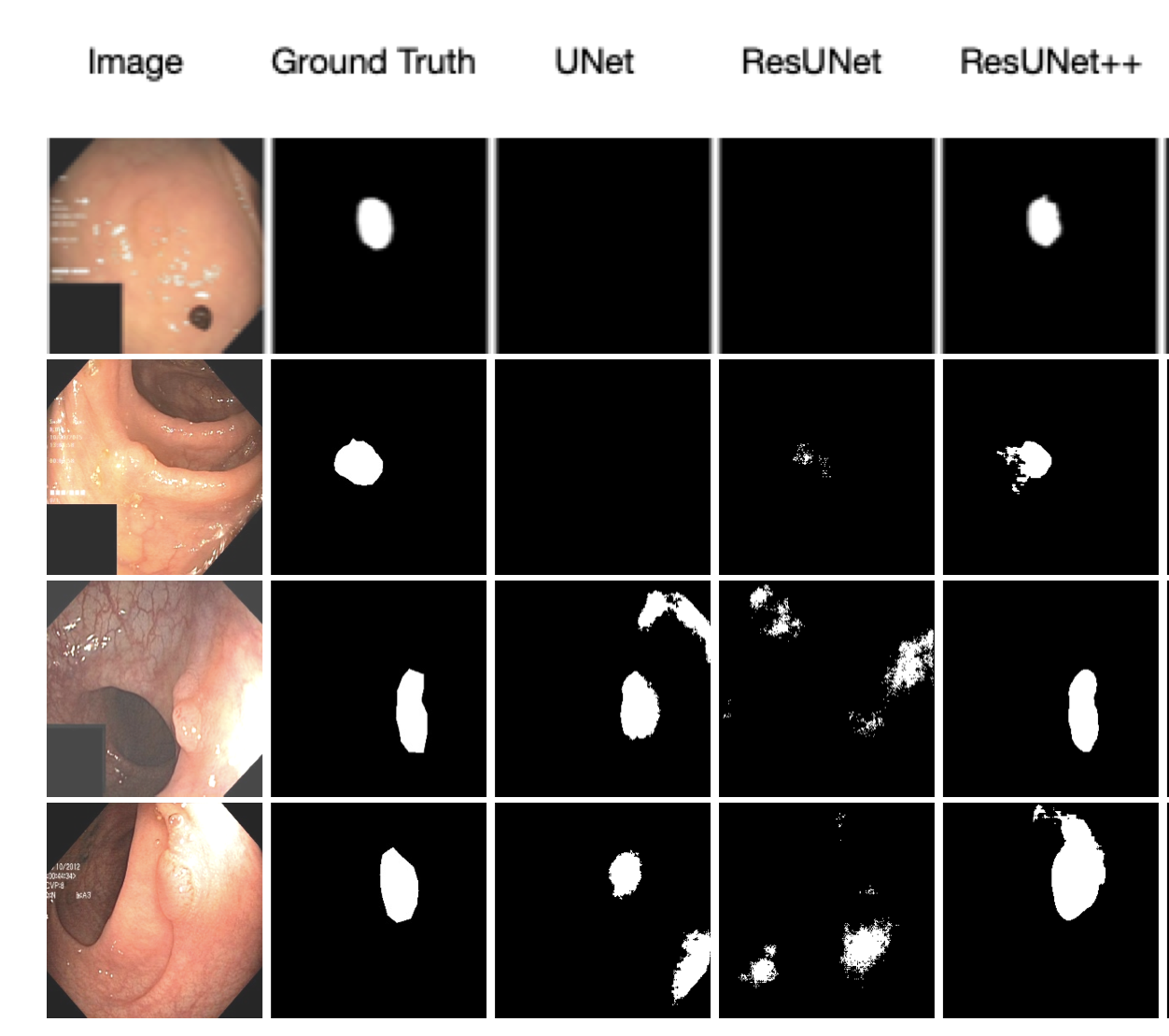 Fig 6. Qualitative result for ResUNet++ [3].
Although still not perfect, we observe the nontrivial differences between predicts by ResUNet++, ResUNet, and UNet. Additionally, we observe that ResUNet+ performance varies a lot when trained without augmented data.
Demo
- Code Base: Drive for VNet
- Code Base: Drive for ResUNet++
- Video: Youtube
References
[1] Milletari, Fausto, Nassir Navab, en Seyed-Ahmad Ahmadi. “V-Net: Fully Convolutional Neural Networks for Volumetric Medical Image Segmentation”. arXiv [cs.CV] 2016.
[2] Imran, Abdullah-Al-Zubaer et al. “Automatic Segmentation of Pulmonary Lobes Using a Progressive Dense V-Network”. Lecture Notes in Computer Science (2018): 282–290.
[3] Jha D, Smedsrud PH, Johansen D, de Lange T, Johansen HD, Halvorsen P, Riegler MA. A Comprehensive Study on Colorectal Polyp Segmentation With ResUNet++, Conditional Random Field and Test-Time Augmentation. IEEE J Biomed Health Inform. 2021 Jun;25(6):2029-2040. doi: 10.1109/JBHI.2021.3049304. Epub 2021 Jun 3. PMID: 33400658.
[4] D. Jha et al., “ResUNet++: An Advanced Architecture for Medical Image Segmentation,” 2019 IEEE International Symposium on Multimedia (ISM), 2019, pp. 225-2255, doi: 10.1109/ISM46123.2019.00049.
[5] D. o. Heresbach, “Miss rate for colorectal neoplastic polyps: a prospec- tive multicenter study of back-to-back video colonoscopies,” Endoscopy, vol. 40, no. 04, pp. 284–290, 2008.