Video Colorization

Historical videos like old movies are all black and white before the invention of colored cameras. However, have you wondered how the good old time looked like with colors? We will attempt to colorize old videos with the power of deep neural networks.

• 1. Introduction
• 2. Problem Formulation
• 3. Image Colorization
  • 3.1 Colorful Image Colorization (2016)
  • 3.2 Instance Aware Image Colorization (2020)
  • 3.3 Blind Video Temporal Consistency via Deep Video Prior (2020)
• 4. Temporal Consistency
  • 4.1 Blind Video Temporal Consistency via Deep Video Prior (2020)
  • 4.2 Deep Exemplar-based Video Colorization
• 5. Metrics
  • 5.1 PSNR
  • 5.2 SSIM
  • 5.3 LPIPS
  • 5.4 Warp Error
• 6. Conclusion
• 7. Demos
  • Video Demo
  • Colab Demo
• 8. Reference

1. Introduction

Colorization is the process of estimating RGB colors from grayscale images or video frames to improve their aesthetic and perceptual quality. Image colorization has been one of the hot-pursuit problems in computer vision research in the past decades. Various models has be proposed that can colorize image in increasing accuracy. Video colorization, on the other hand, remains relatively unexplored, but has been gaining increasingly popularity recently. It inherits all the challenges faced by image colorization, while adding more complexities to the colorization process.

In this project, we will cover some of the state-of-the-art models in video colorization, examine their model architecture, explain their methodology of tackling the problems, and compare their effectiveness. We will also identify the limitations of current models, and shed light on the future course of research in this field.

2. Problem Formulation

Formally, video colorization is the problem where given a sequence of grayscale image frame as input, the model aims to recover the corresponding sequence of RGB image frame. To simplify the problem, we usually adopts YUV channels, where only 2 channels needs to be predicted instead of 3. Video colorization poses the following challenges to the research community:

1. Like image colorization, it is a severely ill-posed problem, as two of the 3 channels are missing. They have to be inferred from other sementics of the image like object detection.

2. Unlike image colorization that only needs to take care of one image at a time, video colorization needs to remain temporally consistent when colorizatoin a sequence of video frames. Directly applying image colorization methods to videos will cause flickering effects.

3. While image colorization is stationary, video colorization has to deal with dynamics scenes, so some frames will be blurred and hard to colorize.

4. Video colorization requires much more computing power than image colorization as the dataset are usually huge and the models are more complex.

3. Image Colorization

To colorize a video, we need to know how to colorize an image first, as a video is essentially a sequence of images. In this section, we explore two image colorization techniques proposed in recent years.

3.1 Colorful Image Colorization (2016)

Introduction paragraph First, we take a look at Zhang’s paper: Colorful Image Colorization [9]. In this paper, the author frames the task of image colorization as finding a mapping \(F: \mathbb{R}^{H\times W \times 1} \to \mathbb{R}^{H \times W \times 2}\). The author uses CIE LAB color space, thereby eliminating the need for predicting a third channel.

The task of colorization requires a special optimization objective. It’s true that the sky is almost always blue, the grass is mostly green, but objects like a beach ball can be of any color. Due to the multimodal nature, using L2 loss leads to the model picking the mean of the modes. This doesn’t result in a good result when the space of plausible coloring is non-convex. Thus, to acquire the colorings, Zhang takes a very convoluted approach.

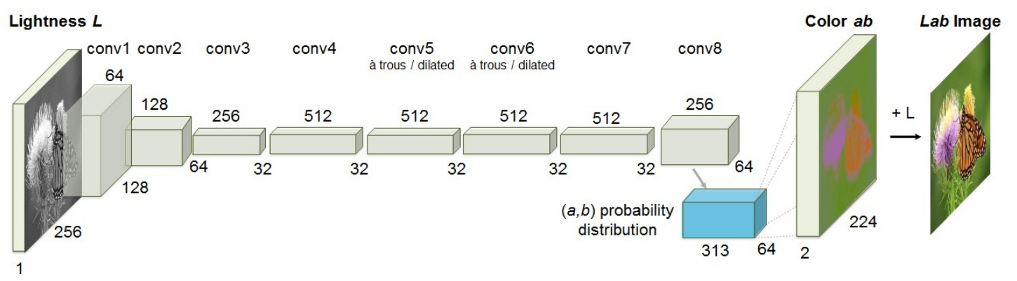
First, using a deep CNN, the author maps the black and white image \(X\) to a possible discrete distribution of the a* b* channels \(\hat{Z}\). The ground truth image \(Y\) is also converted to this space (\(Z\)) using soft-encoding: for each pixel, pick the five closest quantized bins in the a* b* space and weight them proportionally to their distance from the ground truth color. Finally, using a multinomial cross entropy loss, we have our optimization objective:

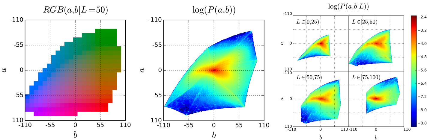
Here, \(v\) returns a weight for each of the possible bins of color. As boring colors are very dominant in ImageNet images, to encourage the model to use vibrant colors, the author assigns a weight that is approximately inversely proportional to the probability of that color in the ImageNet dataset. More formally, for a given color \(q\), the weight \(w \propto ((1-\lambda) P(q) + \frac{\lambda}{Q})^{-1}\), where \(\lambda\) is a parameter and \(Q\) is the number of discrete values in the a* b* space.

Finally, after acquiring a predicted distribution \(\hat{Z}\) in the a* b* space, we need to map it back to \(\mathbb{R}^{H\times W \times 2}\) to find the a* and b* values. For each pixels, picking one of the modes often result in spatial inconsistency, while taking the mean results in a less vibrant result. The author attempts to achieve the best of both worlds by taking an annealed-mean of the distribution:

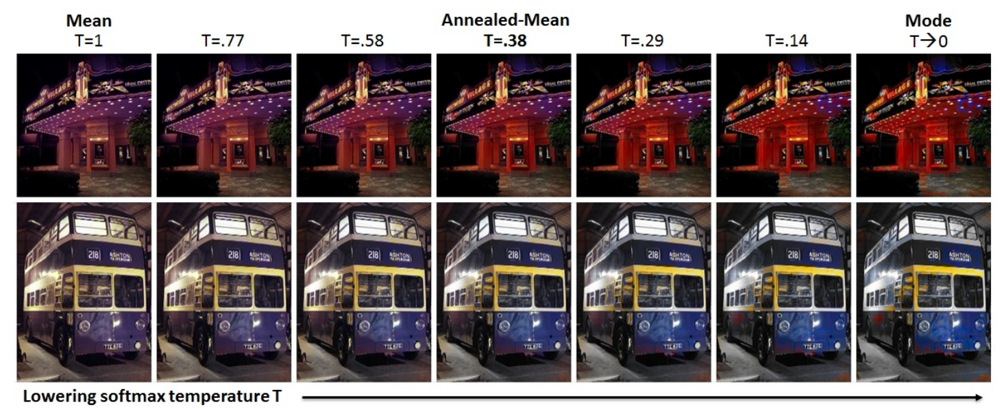
3.2 Instance Aware Image Colorization (2020)

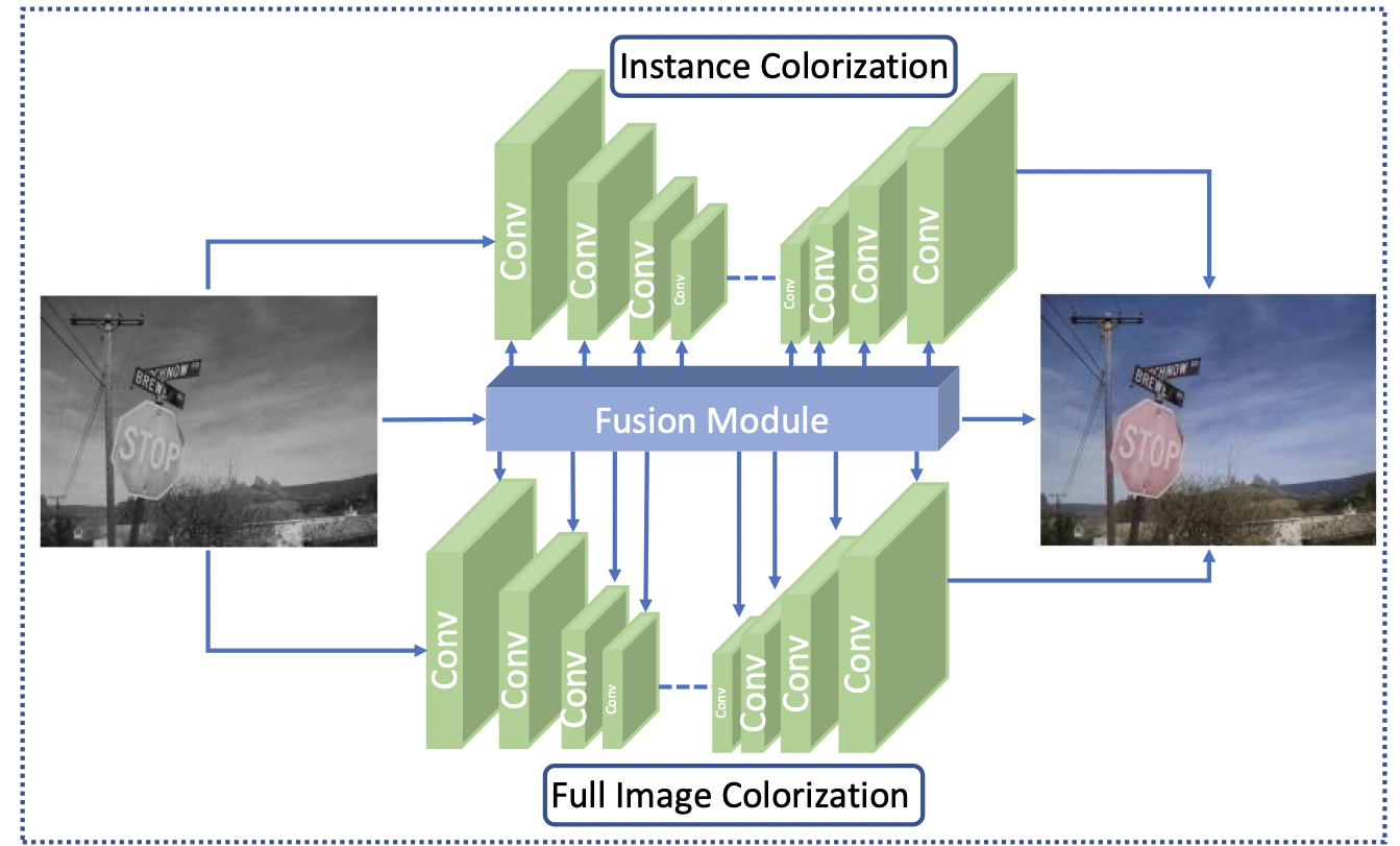
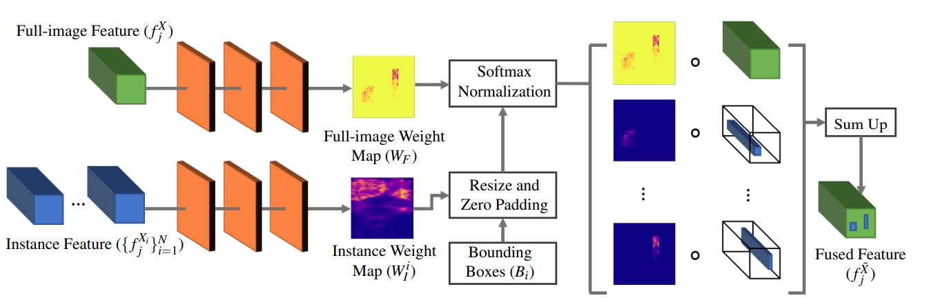
In 2020, Su proposed another way of approaching image colorization [6]. Before the introduction of this paper, image colorization is mostly done in the whole image-level. Previous methods leverage the deep neural network to map input grayscale images to plausible color outputs directly. Arguing that without a clear figure-ground separation, one cannot effectively locate and learn meaningful semantics at object level, this paper proposed a novel network architecture that leverages off-the-shelf models to detect the object, and learn from large-scale data to extract image features at the instance and full-image level, and to optimize the feature fusion to obtain the smooth colorization results. The key insight is that a clear figure-ground separation can dramatically improve colorization performance.

The model consists of three parts, which is shown in figure below:

1. an off-the-shelf pretrained Mask R-CNN model to detect object instances and produce cropped object images.

2. two backbone networks trained end-to-end for instance, and full-image colorization. The paper adopted the main colorization network introduced in Zhang et al. [8] as the backbone network.

3. a fusion module to selectively blend features extracted from different layers of the two colorization networks as shown below. Formally, given a full-image feature \(f^X_j\) and a number of \(N\) of instance features and corresponding object bounding boxes \(\{f^{X_i}_j,B_i\}^N_{i=1}\), we use 2 3-layer CNNs to get full image weight map \(W_F\) and per instance weight map \(W^i_I\) respectively, resize them using the bounding box \(B_i\) to get \(f^{\bar X_i}_j\) and \(\bar W^i_I\), and compute the outputs

3.3 Blind Video Temporal Consistency via Deep Video Prior (2020)

The loss function used in this paper is the smooth \(l_1\) loss with \(\delta=1\):

During the training process, the model is first trained on the full-image colorization, and the weights are transfered to the instance network as initialization, which is then trained. Lastly, both the full iamge and object colorization model are freezed, and the fusion model is trained.

4. Temporal Consistency

Coloring each pixel individually using an image colorization technique often results in color flickering, as the frames do not have a way to “sync up” across time. Thus, we need a method to synchronize the pixel values across the time dimension.

4.1 Blind Video Temporal Consistency via Deep Video Prior (2020)

In 2020, Lei and Xing [3] proposed a novel method to address temporal inconsistency. Unlike Lai’s approach [2], their network does not compute optical flow to establish correspondence. They claimed that the correspondences between frames can be captured implicitly by the visual prior coming from the CNN architecture. As corresponding patches should have similar appearances temporally, they should result in similar CNN outputs.
Moreover, their approach does not require training on massive datasets and can be trained directly on the test video.

The authors approached the problem of temporal inconsistency by first classifying the inconsistency problem into two types:

1. For each pixel location, the pixel values fluctuate around one single value over the entire duration of the video. (unimodal)
2. For each pixel location, the pixel values fluctuate around more than one single value over the entire duration of the video. (multimodal)

To attack the first problem, the authors designed the network shown in Figure 1

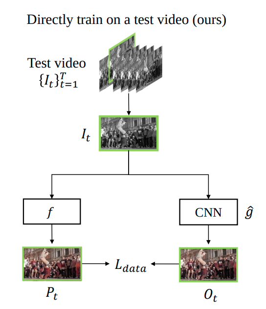
Fig 1. Lei and Xing’s Method.
In each epoch, the model takes in each original black and white frame of the video and passes the frame through both an image colorization algorithm \(f\) and a convolutional autoencoder \(\hat{g}\). The authors used a U-Net[6] for this particular task, and the architectual details are shown in Figure 2. For the purpose of this study, we will explore some other CNN architectures and their efficacy later.
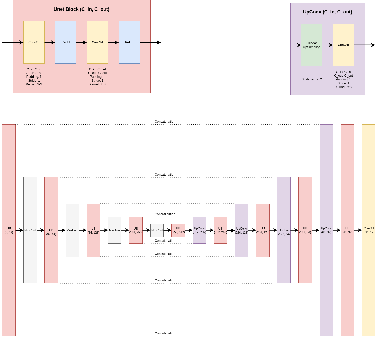Fig 2. Network design.

For the frame \(I_t\) at time step \(t\), we compute \(P_t = f(I_t), O_t = \hat{g}\) and calculate the L1 distance between them. Then, we apply gradient descent to minimize the L1 distance. As we go through the video, the neural net \(\hat{g}\) will approach \(f\). As long as we stop before the neural net overfits, the unimodal inconsistency can be reduced very nicely.

This approach, however, does not solve multimodal inconsistency. As the pixel values cluster around two or more centers, the trained network \(\hat{g}\) would output a value in between all centers (modes). If the modes are far apart, the resulting output color would be far from any of the modes, resulting in a wrong coloring of the frame. To solve this issue, the authors proposed Iteratively Reweighted Training (IRT). Instead of producing one output image from the network, we can produce two output frames, one representing the main mode we want (\(O^{main}_t\)), while the other one represents the other modes that we want to eliminate (outlier frame, \(O^{rest}_t\)). We compute a confidence mask \(C_t\), determining whether a specific pixel on the main frame resembles \(P_t\) more closely than the corresponding pixel on the outlier frame.

Define loss function \(L\) as the follows:

The added degree of freedom allows us to optimize \(O^{main}\) while not compromising correctness to fit multiple modes. In order for the network to actually converge to one of the modes, in practice, we need to go through multiple iterations on the first frame, allowing the network to “grow to like” the mode, and proceed with the rest of the frames.

The Training loop is included below for reference.

for epoch in range(1,maxepoch):
    for id in range(num_of_frames): 
        if with_IRT:      
            # initialize IRT
            if epoch < 6 and ARGS.IRT_initialization:
                # get the I_t and P_t
                net_in,net_gt = frames[0]
                prediction = net(net_in)
                
                # give the main frame a higher weight
                loss = L1(prediction[:,:3,:,:], net_gt) 
                            + 0.9*L1(prediction[:,3:,:,:], net_gt)

            # we've already initialized IRT, proceed with the other frames
            else:
                net_in,net_gt = frames[id]
                prediction = net(net_in)
                
                main_frame = prediction[:,:3,:,:]
                rest_frame = prediction[:,3:,:,:]
                diff_map_main,_ = torch.max(torch.abs(main_frame - net_gt) 
                                    / (net_in+1e-1), dim=1, keepdim=True)
                diff_map_rest,_ = torch.max(torch.abs(rest_frame - net_gt) 
                                    / (net_in+1e-1), dim=1, keepdim=True)
                confidence_map = torch.lt(diff_map_main, 
                                        diff_map_rest)
                                        .repeat(1,3,1,1)
                                        .float()
                crt_loss = L1(main_frame*confidence_map, 
                                net_gt*confidence_map) 
                            + L1(rest_frame*(1-confidence_map), 
                                    net_gt*(1-confidence_map))
        else:
            net_in,net_gt = frames[id] 
            prediction = net(net_in)
            loss = L1(prediction, net_gt)

        optimizer.zero_grad()
        loss.backward()
        optimizer.step()

4.2 Deep Exemplar-based Video Colorization

This work presents the first end-to-end network for exemplar-based video colorization [7], which deals with the temporal consistency problem when colorizing image. Exemplar-based colorization is where the colorization transfers the color from a preconfigured reference image in a similar content to the target grayscale image. But unlike previous exemplar based methods, this work unifies the common separated correspondence and color propagation network, and trained end-to-end to produce more coherent colorization results.

In order to generate temporally consistent videos, DEVC colorize video frames based on the history. Formally, in LAB space, the output is generated as

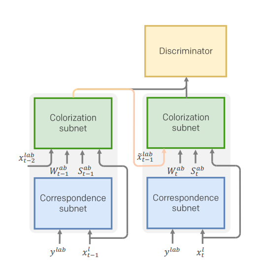
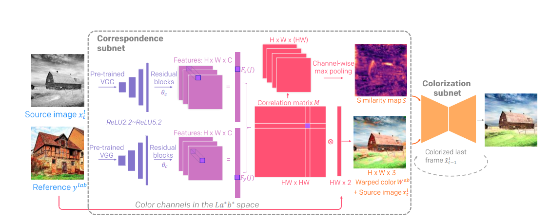
The figure above describes two-stage network architecture. It contains two sub networks.

1. Correspondence Subnet generates two outputs: warped color and confidence map, where \((W^{ab}, S)=N(x^l_t, y^{lab}; \theta_N)\)
2. Colorization Subnet: The correspondence is not accurate everywhere, so we employ the colorization network C which is parameterized by \(\theta_C\), to select the well-matched colors and propagate them properly. The output is formulated as:

Then along with the luminance channel \(x^l_t\), we obtain the final colorized image \(\tilde x_t=\tilde x^{lab}_t\)

DEVC has a quite complicated loss function consisting of 6 parts:

1. Perceptural loss encourages the outputs to be percepturally plausible:

1. Contextual loss encourages the output image to have similar colors with the reference image:

1. Smoothness loss encourages spatial smoothness across the image:

1. Adversarial loss aims to constrain the colorization video frames to remain realistic. In this case, a video discriminator is used to evaluate consecutive video frames, and DEVC adopted a relativistic discriminator that estimates the extent in which the real frames look more realistic than the colorized ones.
2. Temporal consistency loss encourages temporal consistency by penalizes the color change along the flow trajectory:

1. L1 loss to finally encourage similarity between output and target image:

5. Metrics

While human eyes are generally good measuring tools for the effect of colorization models, we still needs some deterministic metrics to quantitatively meaure and compare different models. Researchers have developed several metric t odeal with both colorization and temporal consistency. Here lists a few of them:

5.1 PSNR

PSNR stands for peak signal-to-noise ratio. This metric aims to measure the ratio between the maximum possible power of a signal and the power of corrupting noise that affects the fidelity of its representation. PSNR is commonly used to quantify reconstruction quality for images and video subject to lossy compression, which includes colorization. Given the mean square loss (MSE) between outputs and targets and the MAX possible pixel value of the input image \(MAX_I\), PSNR is defined as:

5.2 SSIM

Then structural similarity index measure (SSIM) is used for measuring the similarity between two images. Given the original image/video and the colorized output, SSIM can be used to measure the fidelity of the color outputted. Given the average of input image \(\mu_y\), and the average and variance of output image \(\mu_{\hat y}\), \(\sigma_{\hat y}\), SSIM is computed as:

Where \({\displaystyle c_{1}=(k_{1}L)^{2}, c_{2}=(k_{2}L)^{2}}\) are two variables to stabilize the division with weak denominator. \({\displaystyle k_{1}=0.01}\) and \({\displaystyle k_{2}=0.03}\) by default. \(L\) is usually set to 1.

5.3 LPIPS

LPIPS measure the perceptual similarity between two image/videos. This work discovered that deep network activations work surprisingly well as a perceptual similarity metric. They therefore constructed deep network for calculating the metric. By linearly “calibrating” networks - adding a linear layer on top of off-the-shelf classification networks including AlexNet, VGG, and SqueezeNet, we can get the metric by directly feeding the outputs into the network.

5.4 Warp Error

Warp error is used to measure the temporal consistency of the colorized video. It measures the spatiotemporal consistency by computing the disparity between every warped previous frame and current frame. It is computed as:

Where \(v_t\) is the generated frame at \(t\) and \(W(O_{t-1\rightarrow t}, v_{t-1})\) is the warped previous frame. \(M_t\) is a binary mask that considers both occlusion regions and motion boundaries.

6. Conclusion

Video colorization is a field that has increasing attention these days. From our experience with this project, current models can have adequate performance on short videos with relative static scenes, but suffers from flickering effect, graying, and color inconsistency when rendering long videos with complex scenes. Therefore, a potential future work is to try making the video more stable for these more complicated videos. Also, as new video dataset has been proposed, like Youtube8M, future works should also consider incorporating these datasets in their training.

7. Demos

Video Demo

Colab Demo

You can go checkout the colab demo at our github repo Colorizer.

8. Reference

[1] Anwar, Saeed, et al. “Image colorization: A survey and dataset.” arXiv preprint arXiv:2008.10774 (2020).
[2] Lai, Wei-Sheng, et al. “Learning blind video temporal consistency.” Proceedings of the European conference on computer vision (ECCV). 2018.
[3] Lei, Chenyang, Yazhou Xing, and Qifeng Chen. “Blind video temporal consistency via deep video prior.” Advances in Neural Information Processing Systems 33 (2020): 1083-1093.
[4] Liu, Yihao, et al. “Temporally Consistent Video Colorization with Deep Feature Propagation and Self-regularization Learning.” arXiv preprint arXiv:2110.04562 (2021).
[5] Ronneberger, Olaf, Philipp Fischer, and Thomas Brox. “U-net: Convolutional networks for biomedical image segmentation.” International Conference on Medical image computing and computer-assisted intervention. Springer, Cham, 2015.
[6] Su, Jheng-Wei, Hung-Kuo Chu, and Jia-Bin Huang. “Instance-aware image colorization.” Proceedings of the IEEE/CVF Conference on Computer Vision and Pattern Recognition. 2020.
[7] Zhang, Bo, et al. “Deep exemplar-based video colorization.” Proceedings of the IEEE/CVF Conference on Computer Vision and Pattern Recognition. 2019.
[8] Zhang, Richard, et al. “Real-time user-guided image colorization with learned deep priors.” arXiv preprint arXiv:1705.02999 (2017).
[9] Zhang, Richard, Phillip Isola, and Alexei A. Efros. “Colorful image colorization.” European conference on computer vision. Springer, Cham, 2016.