DeepFake Generation
This is the blog that records and explains technical details for Chenda Duan and Zhengtong Liu’s CS188 DLCV project. We investigate some novel and powerful methods of two topics in DeepFake Generation: Image Animation and Image-to-Image Translation methods. For better understanding and for fun, we have create a demo. You may need to create a copy and modify the path in the deepFake_demo.ipynb file.
- What is DeepFake?
- Core ideas: GAN
- Image Animation
- Image-to-Image Translation
- Video Demo
- Colab Demo
- Relevant Papers
What is DeepFake?
What is DeepFake? Originally, it was a term created by some reddit users. It now refers to using deep learning to generate “fake” images, which look like photos captured in the real world but is not.
The most heated use of deep fake is to do the face swapping, which is the subset of a broader definition called “DeepFake generation”. As you might see in recent years, more and more people get access to well-performed deep fake algorithms and create funny, weird images that might even cause problems.
Here is an example of using DeepFake generation:
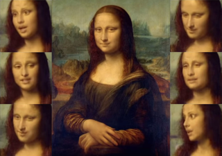
Fig 1. A example of DeepFake generation. (Image source: https://news.artnet.com/art-world/mona-lisa-deepfake-video-1561600)
As DeepFake generation might cause many problems (such as fake news!), the other popular sub-topic is DeepFake detection, where we try to build the network that can identify real images from fake, generated images.
Core ideas: GAN
GAN (“Generative adversarial network”) is the core framework behind most of the DeepFake algorithms. The idea is simple, for DeepFake generators, the more easily you can trick the human eyes, the better your algorithm is. And for the DeepFake detector, the more easily you can detect the fake image, the better. However, we cannot train a DeepFake generators by manually evaluating how good the result is, and we need the help of the detector.
That brings the idea of “adversarial”: the generator tries to fool the detector, and the detector tries to detect every fake image produced by the generator. And we train these two network at the same time.
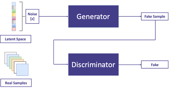
Fig 2. A simple structure for GAN network. (Image source: https://neptune.ai/blog/6-gan-architectures)
Below we mainly focus on two applications, Image Animation and Image-to-Image Translation, of the DeepFake generation.
Image Animation
Image Animation is interesting in that it produces animation of an object from a static image. Here we introduce a self-supervised image animation framework called the First Order Motion Model. We mainly focus on the architecture of this model, as well as the mathematical formulation behind each step. We also briefly touch on other methods of Image Generation, and discuss a bit about the pros and cons of each method.
First Order Motion Model for Image Animation
The First Order Motion Model animates an object in the source image according to the motion of a driving video. The method uses self-learned keypoints together with local affine transformations to model complex motions. (Therefore, they call this method a first-order method.) Note that they uses an occlusion-aware generator and extends the equivariance constraint, commonly used for keypoints detection training, to improve the estimation of local affine transformations.

Fig 3. First Order Motion Model on VoxCeleb Dataset. (Image source: https://github.com/AliaksandrSiarohin/first-order-model/blob/master/sup-mat/vox-teaser.gif)
The framework consists of two modules: the motion estimation module and the image generation module. The motion estimation module predicts a dense motion field from a frame \(\mathbf{D} \in \mathbb{R}^{3 \times H \times W}\) of the driving video \(\mathcal{D}\) to the source frame \(\mathbf{S} \in \mathbb{R}^{3 \times H \times W}\). The backward optical flow \(T_{S \leftarrow D}\) is used since backward-warping can be implemented efficiently using bilinear sampling. Also, they assume an abstract reference frame, \(\mathbf{R}\), which cancels in the later derivations and never explicitly computed, to allow for independent process of \(\mathbf{D}\) and \(\mathbf{S}\).
The motion estimation module is divided to two steps. In the first step, the sparse motion representation is approximated using keypoints and local affine transformations. Keypoint locations in \(\mathbf{D}\) and \(\mathbf{S}\) are predicted separately by an encoder-decoder network. To model a larger familiy of transformations, they use Taylor expansion to represent \(T_{D \leftarrow R}\) by a set of keypoint locations and affine transformations. For a given frame \(\mathbf{X}\), and a set of keypoint coordinates \(p_1, \ldots, p_K\), the motion function \(T_{X \leftarrow R}\) is represented by its value in each keypoint \(p_k\) and its Jacobian computed in each \(p_k\) location:
\[T_{X \leftarrow R} \simeq \left\{ \left\{ T_{X \leftarrow R} (p_1), \frac{d}{dp} T_{X \leftarrow R}(p) \bigg\rvert_{p = p_1}\right\}, \ldots, \left\{ T_{X \leftarrow R} (p_K), \frac{d}{dp} T_{X \leftarrow R}(p) \bigg\rvert_{p = p_K}\right\}\right\}\]To estimate \(T_{S \leftarrow D}\) at keypoint \(z_k\) in \(\mathbf{D}\) such that \(p_k = T_{R \leftarrow D} (z_k)\) (so \(z_k = T_{D \leftarrow R} (p_k)\)), we have
\[\begin{equation*} \begin{split} T_{S \leftarrow D} (z_k) &= T_{S \leftarrow R} \circ T_{R \leftarrow D} (z_k) \\ &= T_{S \leftarrow R } \circ T^{-1}_{D \leftarrow R} (z_k)\\ &= T_{S \leftarrow R } \circ T^{-1}_{D \leftarrow R} T_{D \leftarrow R} (p_k) \\ &= T_{S \leftarrow R} (p_k) \end{split} \end{equation*}\]Using the first order Taylor expansion of \(T_{S \leftarrow R} (p_k)\) at \(p_k\), we get
\[\begin{equation*} \begin{split} T_{S \leftarrow D}(z) &= T_{S \leftarrow R} (p_k)\\ &\approx T_{S \leftarrow R} (p_k) + \left( \frac{d}{dp} T_{S \leftarrow D}(p) \bigg\rvert_{p = p_k} \right)\\ &= T_{S \leftarrow R} (p_k) + \left( \frac{d}{dp} T_{S \leftarrow R} (p) \bigg\rvert_{p = p_k} \right) \left( \frac{d}{dp} T_{D \leftarrow R} (p) \bigg\rvert_{p = p_k} \right)^{-1} (z - T_{D \leftarrow R} (p_k)) \end{split} \end{equation*} \label{eq1}\tag{1}\]where \(T_{S \leftarrow R}\) and \(T_{D \leftarrow R}\) are predicted by the keypoint predictor (a standard U-Net that estimates \(K\) heatmaps, one for each keypoint). Note that equivaraince constraints are imposed when training the keypoint predictor. The deformed images (thin plate spline deformations, specifically) are passed as the inputs to force the model to predict consistent keypoints with respect to known geometric transformations. As shown below, the equivariance loss involves constraints on keypoints as well as on the Jacobians. Suppose an image \(\mathbf{X}\) is deformed to \(\mathbf{Y}\) under the transformation \(T_{X \leftarrow Y}\), the constraints used in this model are
\[T_{X \leftarrow R} \equiv T_{X \leftarrow Y} \circ T_{Y \leftarrow R} (p_k) \\ \mathbb{1} \equiv \left(\frac{d}{dp} T_{X \leftarrow R}(p) \bigg\rvert_{p = p_k} \right)^{-1} \left(\frac{d}{dp} T_{X \leftarrow Y}(p) \bigg\rvert_{p = T_{Y \leftarrow R}(p_k)} \right) \left(\frac{d}{dp} T_{Y \leftarrow R}(p) \bigg\rvert_{p = p_k} \right)\]Below are the code snip showing the structrues of the keypoint detector.
def forward(self, x):
    if self.scale_factor != 1:
        x = self.down(x)

    feature_map = self.predictor(x)
    prediction = self.kp(feature_map)

    final_shape = prediction.shape
    heatmap = prediction.view(final_shape[0], final_shape[1], -1)
    heatmap = F.softmax(heatmap / self.temperature, dim=2)
    heatmap = heatmap.view(*final_shape)

    out = self.gaussian2kp(heatmap)

    if self.jacobian is not None:
        jacobian_map = self.jacobian(feature_map)
        jacobian_map = jacobian_map.reshape(final_shape[0], self.num_jacobian_maps, 4, final_shape[2],
                                            final_shape[3])
        heatmap = heatmap.unsqueeze(2)

        jacobian = heatmap * jacobian_map
        jacobian = jacobian.view(final_shape[0], final_shape[1], 4, -1)
        jacobian = jacobian.sum(dim=-1)
        jacobian = jacobian.view(jacobian.shape[0], jacobian.shape[1], 2, 2)
        out['jacobian'] = jacobian

    return out
In the second step, a dense motion network combines the local approximations to estimate the dense motion field \(\hat{T}_{S \leftarrow D}\). The source frame \(\mathbf{S}\) is warped according to Eq. (\(\ref{eq1}\)) to obtain \(K\) transformed images \(\mathbf{S^1}, \ldots \mathbf{S^K}\), so that the inputs are roughly aligned with \(\hat{T}_{S \leftarrow D}\) when prediction from \(S\) (\(\hat{T}_{S \leftarrow D}\) aligns local patterns with pixels in \(\mathbf{D}\) not \(\mathbf{S}\)). The heatmaps \(\mathbf{H_k}\), which indicates where each transformation happens, are calculated as below:
\[\mathbf{H}_z (z) = \exp\left(\frac{(T_{D \leftarrow R} (p_k) - z)^2}{\sigma}\right) - \exp\left(\frac{(T_{S \leftarrow R} (p_k) - z)^2}{\sigma}\right)\]Then the \(\mathbf{H_k}\) and the transformed images \(\mathbf{S}^{1} \ldots \mathbf{S}^{K}\), as well as the original image \(\mathbf{S}^{0} = \mathbf{S}\) considered for the background, are passed to a U-Net, from which \(K+1\) masks \(\mathbf{M}_k, k = 0, \ldots, K\) are estimated to indicate where each local transformation holds. Then the final dense motion prediction \(\hat{T}_{S \leftarrow D} (z)\) is
\[\begin{equation} \begin{split} \hat{T}_{S \leftarrow D} (z) &= \mathbf{M}_0 z + \displaystyle{\sum_{k = 1}^k \mathbf{M}_k \hat{T}_{S \leftarrow R} (p_k)}\\ &= \mathbf{M}_0 z + \displaystyle{\sum_{k = 1}^k \mathbf{M}_k \left(T_{S \leftarrow R} (p_k) + \left( \frac{d}{dp} T_{S \leftarrow R} (p) \bigg\rvert_{p = p_k} \right) \left( \frac{d}{dp} T_{D \leftarrow R} (p) \bigg\rvert_{p = p_k} \right)^{-1} (z - T_{D \leftarrow R} (p_k))\right)} \end{split} \end{equation}\]Since image-warping according to the optical flow may not work in the presence of occlusion in \(\mathbf{S}\), the occlusion map is used to mask out the feature map regions that need to be impainted. Therefore, the occlusion mask \(\hat{\mathcal{O}}_{S \leftarrow D}\) is estimated by adding a channel to the final layer of the dense motion netowrk.
After the the motion estimation module, the generation module is quite straightforward. A generation netowrk is trained to warp the source image according to \(\hat{T}_{S \leftarrow D}\) an inpaint the image parts that are occluded in the source image. It is worth to notice, however, that the first-order model uses the relative motion transfer in the testing stage. Instead of transforming each frame of the driving video \(\mathbf{D}_t\) to \(\mathbf{S}_t\) directly in animation of an object in the source frame \(\mathbf{S}_1\), they transfer the transfer the relative motion between \(\mathbf{D}_1\) and \(\mathbf{D}_t\) to \(\mathbf{S}_1\). For the neighborhood of each keypoint \(p_k\) of \(D_1\), \(T_{D_t \leftarrow D_1} (p)\) is applied:
\[\displaystyle{T_{S_1 \leftarrow S_t} (z) \approx T_{S_1 \leftarrow R} (p_k) + \left(\frac{d}{dp} T_{D_1 \leftarrow R} (p) \bigg\rvert_{p = p_k} \right) \left(\frac{d}{dp} T_{D_t \leftarrow R} (p) \bigg\rvert_{p = p_k} \right)^{-1} (z - T_{S \leftarrow R} (p_k) + T_{D_1 \leftarrow R}(p_k) - T_{D_t \leftarrow R}(p_k))}\]This equation can actually be derived from Eq. (\(\ref{eq1}\)). Note that one assumption of the first-order model is that \(\mathbf{S_1}\) and \(\mathbf{D_1}\) have similar poses. Otherwise, the idea of relative motion transfer here might not work.
Below are the code snip showing the structures of the image generation module, you can see the dense motion network and the occulusion mask mentioned above.
def forward(self, source_image, kp_driving, kp_source):
        # Encoding (downsampling) part
        out = self.first(source_image)
        for i in range(len(self.down_blocks)):
            out = self.down_blocks[i](out)

        # Transforming feature representation according to deformation and occlusion
        output_dict = {}
        if self.dense_motion_network is not None:
            dense_motion = self.dense_motion_network(source_image=source_image, kp_driving=kp_driving,
                                                     kp_source=kp_source)
            output_dict['mask'] = dense_motion['mask']
            output_dict['sparse_deformed'] = dense_motion['sparse_deformed']

            if 'occlusion_map' in dense_motion:
                occlusion_map = dense_motion['occlusion_map']
                output_dict['occlusion_map'] = occlusion_map
            else:
                occlusion_map = None
            deformation = dense_motion['deformation']
            out = self.deform_input(out, deformation)

            if occlusion_map is not None:
                if out.shape[2] != occlusion_map.shape[2] or out.shape[3] != occlusion_map.shape[3]:
                    occlusion_map = F.interpolate(occlusion_map, size=out.shape[2:], mode='bilinear')
                out = out * occlusion_map

            output_dict["deformed"] = self.deform_input(source_image, deformation)

        # Decoding part
        out = self.bottleneck(out)
        for i in range(len(self.up_blocks)):
            out = self.up_blocks[i](out)
        out = self.final(out)
        out = F.sigmoid(out)

        output_dict["prediction"] = out

        return output_dict
Global-Flow Local-Attention Model
Although the first-order motion model achieves pretty good performance, it actually leads to compromised results in some cases. For example, we tried to set the images of ourselves as the source image. However, the keypoints detection were not accurate and the animation result looks unnatuaral in some cases, especially when the source image is not cropped to roughly align with the driving video.
Additionally, for the first order motion model, the pretrained model is highly sensitive and only works well on the images similar to its training set. If, for exmaple, the model is trained on face images, then the model will perform poorly for images where the face only takes up a small portion. (To try out yourself, the Colab demo we provide might be helpful.)
Here we also introduce another framework that can accomplish the Image Animation task, the Global-Flow Local-Attention Model. Similar to the first-order motion model, this framework composes of two parts: Global Flow Field Estimator and Local Neural Texture Renderer. The Global Flow Field Estimator employs a flow-based method to extract the global correlations and generate flow fields, while the Local Neural Texture Renderer uses a local-attention mechanism to spatially transform the information from the source to target. Below shows a example video generated from the source image. Since this method is originally proposed for the task of pose-guided person image generation, edge guidance is also shown. (resolution of the demo slightly compromised when converting from video to gif)
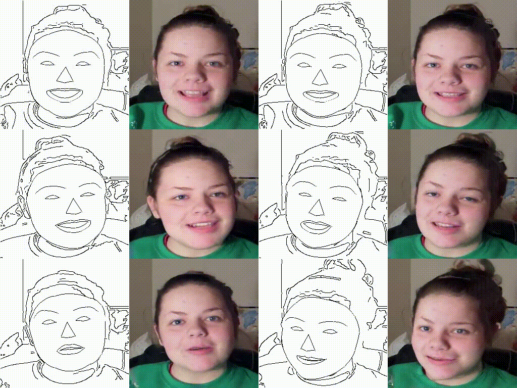
Fig 4. A demo of the Global-Flow-Local-Attention model application on image animation.(Video source: https://drive.google.com/file/d/1YJfGzpCZ0ZDtbyRrEEBXtH-qSHHB8ltT/view?usp=sharing)
However, this method also has some drawbacks. This method requires an explicit edge guidance video. This edge guidance video is processed from a sequence of source images in the demo provided. While this method generates videos with vivid details, it also require more source images in some sense.
We do not provide a detailed explanation of the Global-Flow Local-Attention framework here. Readers who are interested in this method may refer to the original paper.
Image-to-Image Translation
Image-to-Image Translation has been a popular topic in DeepFake generation. As we learned in class, StyleGAN v3 is the current state-of-the-art method. In this part, we choose to mainly introduce a novel method called StarGAN (particularly, StarGAN v2). This model adopts many ideas from previous works. Therefore, we will introduce interesting methods used in StarGAN v2 model aside from StarGAN v2 itself below, which hopefully can help the readers to have a more comprehensive view of this model and the Image-to-Image Translation field as a whole.
StarGAN v2: Diverse Image Synthesis for Multiple Domains
The StarGAN v2 model is an image-to-image translation framework that can generate diverse images of multiple domains with good scalibility. In this paper, domain refers to a set of images that can be grouped as a visually distinctive category (e.g. images of cats and dogs can be two domains); while style means a unqiue appearance of an image (e.g. hairstyle). Briefly speaking, this framework uses domain-specific decoders to interpret latent style codes to achieve style diversity, and the generator takes an additional domain information so that images of multiple domains can be handled using a single framework. Next, we introduce StarGAN v2 from the framework and the learning objective functions.

Fig 5. StarGAN v2 on CelebA-HQ Dataset. (Image source: https://github.com/clovaai/stargan-v2/blob/master/assets/celebahq_interpolation.gif)
- Framework
-
Generator \(G(\mathbf{x}, \mathbf{s})\) generates an image with an input image \(\mathbf{x}\) and style code \(\mathbf{s}\). Notice that \(G\) deviates from the origianl GAN model in that it takes in two inputs. This formulation was first proposed in Image-to-Image Translation with Conditional Adversarial Networks as conditional GANs (cGANs) are suitable for image-to-image generation tasks, in which we generate an image conditioning on a source image (in this case, image \(\mathbf{x}\)).
The style code \(\mathbf{s}\) is injected into \(G\) according to the adpative instance normalization (AdaIN). AdaIN is a method that aligns the mean and varaiance of the input features with those of the style features, which is more efficient and simpler than the traditional style swap layer. The idea can be tracked back to Arbitrary Style Transfer in Real-time with Adaptive Instance Normalization and was adopted by the state-of-art image style transfer method StyleGAN. Specifically in this case, the AdaIN operation is defined as
\[\mathrm{AdaIN}(x_i, s) = \sigma(s) \left( \frac{x_i - \mu{(x)}}{\sigma{(x)}} \right) + \mu(s)\]where \(x_i\) is some feature map at some layer of \(G\). Here we also provide a figure from StyleGAN to demonstrate the use of AdaIN. In the right figure, “A” represents the learned affined transform (in this paper, \(\sigma(s)\) and \(\mu(s)\)) and “B” applies learned scaling factors to the noise (in StyleGAN model);
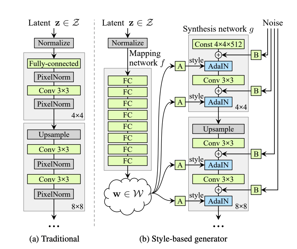
Fig 6. Demonstration of AdaIN operation. (Image source: https://arxiv.org/pdf/1812.04948.pdf)
Below are the structures of the generators:
def forward(self, x, s, masks=None): x = self.from_rgb(x) cache = {} for block in self.encode: if (masks is not None) and (x.size(2) in [32, 64, 128]): cache[x.size(2)] = x x = block(x) for block in self.decode: x = block(x, s) if (masks is not None) and (x.size(2) in [32, 64, 128]): mask = masks[0] if x.size(2) in [32] else masks[1] mask = F.interpolate(mask, size=x.size(2), mode='bilinear') x = x + self.hpf(mask * cache[x.size(2)]) return self.to_rgb(x) ## Note that the self.encode and self.decode contains the AdaIN blocks mention above for _ in range(2): self.encode.append( ResBlk(dim_out, dim_out, normalize=True)) self.decode.insert( 0, AdainResBlk(dim_out, dim_out, style_dim, w_hpf=w_hpf)) if w_hpf > 0: device = torch.device( 'cuda' if torch.cuda.is_available() else 'cpu') self.hpf = HighPass(w_hpf, device) -
Mapping network \(F_y(\mathbf{z})\) takes in a latent code \(\mathbf{z}\) outputs a style code \(s\) corresponding to the domain \(y\). \(F\) can produce diverse style codes by sampling \(z \in \mathcal{Z}\) and \(y \in \mathcal{Y}\) randomly.
-
Style encoder \(E_y(\mathbf{x})\) extracts the style code \(\mathbf{s}\) corresponding to the domain \(y\) from the image \(x\). Like the mapping network \(F\), \(E\) can also produce style codes of different domains and reference images.
-
Discriminator \(D\) is a multitask discriminator consisting of multiple output branches. Each branch \(D_y\) learns to classifies whether an image \(\mathbf{x}\) is a real image of domain \(y\) or a fake image generated by \(G\).
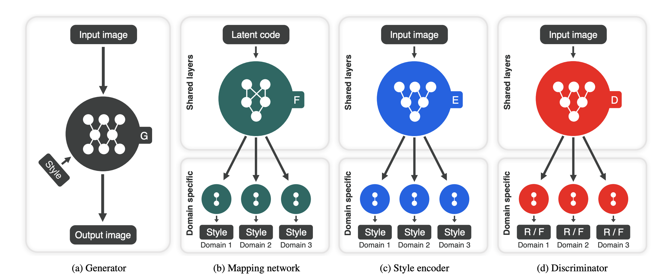
Fig 7. Overview of StarGAN v2 framework. (Image source: https://arxiv.org/pdf/1812.04948.pdf)
-
- Learning objective functions
Notations that we will use below: an input image \(\mathbf{x} \in \mathcal{X}\) and its original domain \(\mathbf{y} \in \mathcal{Y}\); a latent code \(\mathbf{z} \in \mathcal{Z}\); a target domain \(\tilde{y} \in \mathcal{Y}\) and style code \(\tilde{\mathbf{s}}\).-
Adversarial objective
\[\mathcal{L}_{adv} = \mathbb{E}_{\mathbf{x}, y}[\log{D_y(\mathbf{x})}] + \mathbb{E}_{\mathbf{x}, \tilde{y}, \mathbf{z}}[\log{(1 - D_{\tilde{y}} (G(\mathbf{x}, \tilde{\mathbf{s}})))}]\]where the latent code \(\mathbf{z}\) and target domain \(\tilde{y}\) are sampled randomly in training and \(\tilde{s} = F_{\tilde{y}}(\mathbf{z})\).
Below are the code snip defining the adversarial loss:
def adv_loss(logits, target): assert target in [1, 0] targets = torch.full_like(logits, fill_value=target) loss = F.binary_cross_entropy_with_logits(logits, targets) return loss -
Style reconstruction
\[\mathcal{L}_{sty} = \mathbb{E}_{\mathbf{x}, \tilde{y}, \mathbf{z}}[\|\tilde{\mathbf{s}} - E_{\tilde{y}} (G(\mathbf{x}, \tilde{\mathbf{s}})) \|]_{1}\]This loss function says that the we should be able to reconstruct the style code \(\tilde{\mathbf{s}}\) by encoding the generated image with style code input as \(\tilde{\mathbf{s}}\) itself. This forces the generator \(G\) to make use of the style code \(\tilde{\mathbf{s}}\) when generating the image \(G(\mathbf{x}, \tilde{\mathbf{s}})\).
Such reconstruction loss is common used in multimodal image-to-image translation, where images are often encoded as the latent code in the low dimension based on the partially shared latent space assumption made in Multimodal Unsupervised Image-to-Image Translation, that each image \(\mathbf{x} \in \mathcal{X}\) is generated from a content latent code \(c \in \mathcal{C}\) that is shared across domains, and a style latent code \(\mathbf{s} \in \mathcal{S}\) that is specific to the individual domain. Therefore, the encoder-decoder structure, with style code injected, can be justified. In Fig. 7, we see that the reconstruction loss can be computed between images and between latent codes (we only use reconstruction loss between style codes in StarGAN v2).
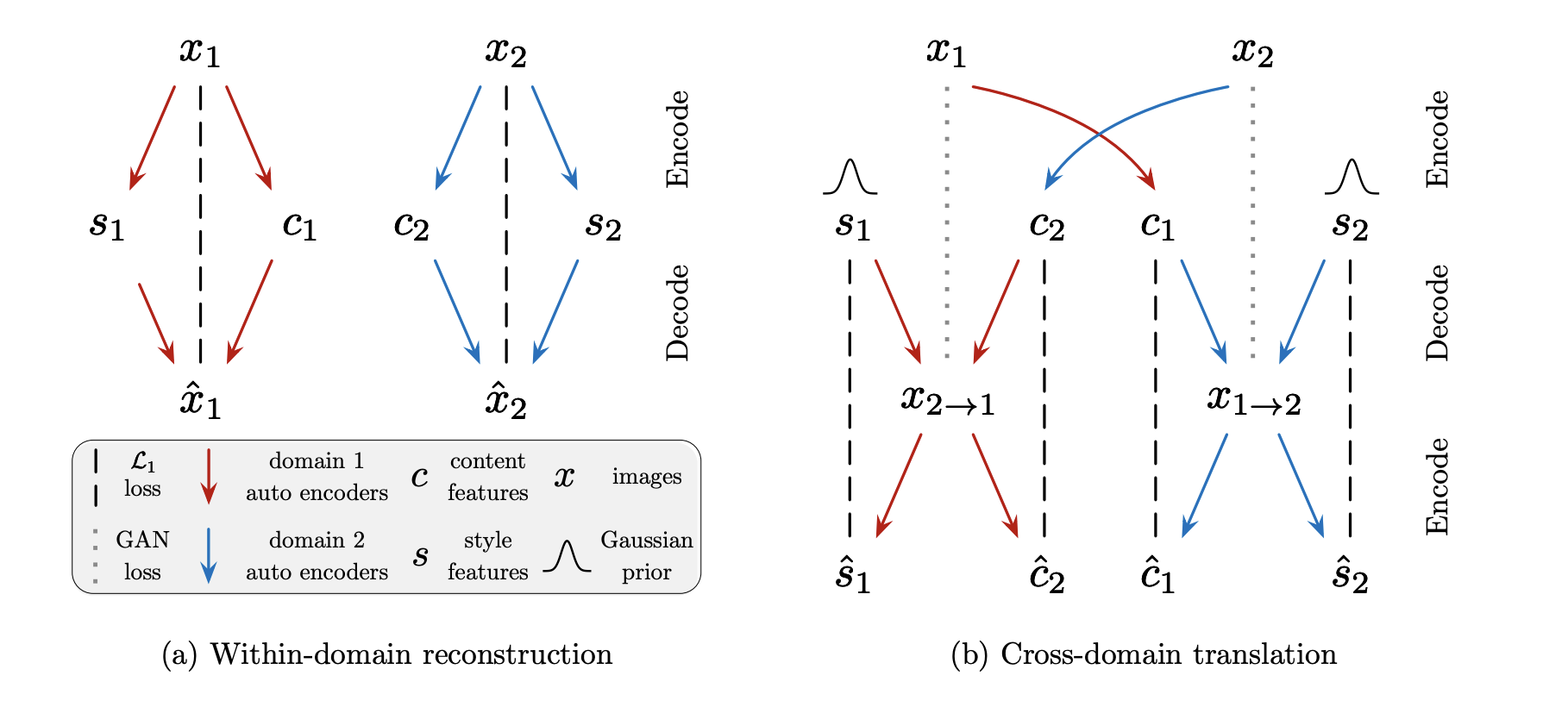
Fig 8. Reconstruction Loss in Multimodal Unsupervised Image-to-Image Translation. (Image source: https://arxiv.org/pdf/1804.04732.pdf)
Below are the code snip defining the Style reconstruction loss:
s_pred = nets.style_encoder(x_fake, y_trg) loss_sty = torch.mean(torch.abs(s_pred - s_trg)) -
Style diversification
\[\mathcal{L}_{ds} = \mathbb{E}_{\mathbf{x}, \tilde{y}, \mathbf{z}_1, \mathbf{z}_2} [\| G(\mathbf{x}, \tilde{\mathbf{s}}_1) - G(\mathbf{x}, \tilde{\mathbf{s}}_2) \|_1]\]where \(\mathbf{z}_1, \mathbf{z}_2\) are two random latent codes and \(\tilde{s}_{i} = F_{\tilde{y}}(\mathbf{z}_{i})\) for \(i \in {1, 2}\). It is worth noticing that we want to maximize instead of minimizing this objective function, as we encourage the generator \(G\) to disversify the output images according to the target style codes. This syle diversification regularization term was first introduced in Mode Seeking Generative Adversarial Networks for Diverse Image Synthesis. The mode collapse issue for cGANs, that generators tend to ignore the input noisy vectors but focus on the prior conditional information provided, makes the generator more prone to produce images with similar appearances. Motivated by this, the mode seeking GAN model was proposed, in which the style diversification regularization term was added to encourage the generator to explore the image spaces and enhance the chances of generating images from minor modes.
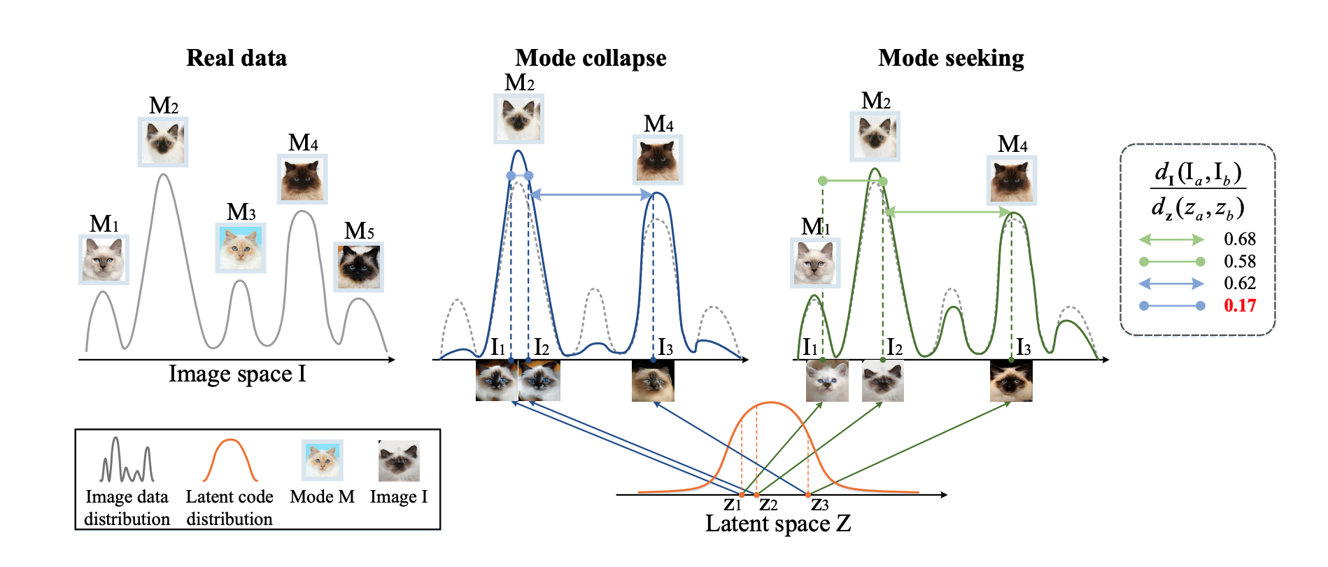
Fig 9. Illustration of mode collapose. (Image source: https://arxiv.org/pdf/1903.05628.pdf)
While original regularization term has the difference \(\|\mathbf{z}_1 - \mathbf{z}_2 \|_1\) in the denominator, the StarGAN v2 model removes this for the sake of stability of training process (the difference \(\|\mathbf{z}_1 - \mathbf{z}_2 \|_1\) is small and thus increase the loss significantly).
Below are the code snip defining the Style diversification loss:
if z_trgs is not None: s_trg2 = nets.mapping_network(z_trg2, y_trg) else: s_trg2 = nets.style_encoder(x_ref2, y_trg) x_fake2 = nets.generator(x_real, s_trg2, masks=masks) x_fake2 = x_fake2.detach() loss_ds = torch.mean(torch.abs(x_fake - x_fake2)) -
Preserving source characteristics
\[\mathcal{L}_{cyc} = \mathbb{E}_{\mathbf{x}, y, \tilde{y}, \mathbf{z}}[\| \mathbf{x} - G(G(\mathbf{x}, \tilde{\mathbf{s}}), \hat{\mathbf{s}})\|_{1}]\]where \(\hat{\mathbf{s}} = E_y(\mathbf{x})\) is the estimated style code of the input image \(\mathbf{x}\). By minimizing this objective function, we want to make sure that the generator can preserve the domain-invariant characteristics.
This cycle consistency loss, while was already adopted in the previous version of StyleGAN, was used extensively in another well-known method in the field of image-to-image transfer, called CycleGAN. In the paper Unpaired Image-to-Image Translation using Cycle-Consistent Adversarial Networks, the cylce consistency loss is utilized to ensure that \(F(G(X)) \approx X\), where \(G: X \to Y\) and \(F: Y \to X\) are two learnable mappings to generate paired images with no paired training data.

Fig 10. Illustration of Cylce Consistency Loss. (Image source: https://arxiv.org/pdf/1703.10593.pdf)
Below are the code snip defining the cycle consistency loss
  masks = nets.fan.get_heatmap(x_fake) if args.w_hpf > 0 else None
  s_org = nets.style_encoder(x_real, y_org)
  x_rec = nets.generator(x_fake, s_org, masks=masks)
  loss_cyc = torch.mean(torch.abs(x_rec - x_real))
Combine the above objectives, the full objective is
\[\min_{G, F, E} \max_{D} \mathcal{L}_{adv} + \lambda_{sty} \mathcal{L}_{sty} - \lambda_{ds} \mathcal{L}_{ds} + \lambda_{cyc} \mathcal{L}_{cyc}\]where \(\lambda_{sty}\), \(\lambda_{ds}\) and \(\lambda_{cyc}\) are hyperparamters for the regularization terms. Below are the code snip showing the overall loss functions:
loss = loss_adv + args.lambda_sty * loss_sty \ - args.lambda_ds * loss_ds + args.lambda_cyc * loss_cyc -
StyleGAN: Synthesize the Style
Learning about StarGAN, and how it uses AdaIN to fuse the style features and the input features, we will breifly introduce the first work that propose AdaIN: StyleGAN.
We know that for traiditonal GAN, the generator ususally takes a randomly generated latent vector and generates the images. However, people actually have little control over the latent vector. What if, say, we want to fuse two images, and take one image’s overall looks and the other image’s styles? We cannot brute-forcely add up, or take the mean of, their latent vector. We need to somehow disentangle the parts of the vector that controls the style.
So that’s the reason of the StyleGAN and its AdaIN. The general architure of the generator of StyleGAN is already list above (when introducing the AdaIN). The basic idea is that, different part of the generators (4x4 and 8x8) controls different features. The paper mentioned that the first half of the generator controls more on the overall looks of the images (i.e, male or female), whereas the latter part of the network controls more on the style (hair, glasses, expressions). Thus, by feeding two style vectors from different source images, we can essentially fuse the style of one images into the other.
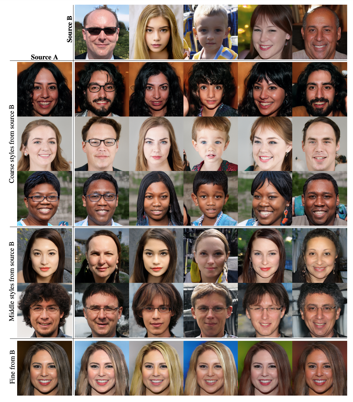
Fig 11. Demo for StyleGAN. (Image source: https://arxiv.org/pdf/1812.04948.pdf)
No one is perfect, and so does the GAN. There are some drawbacks for the networks we mentioned. Note some of them are found by ourselves and may not being well-analyzed.
For StarGAN, according to the analysis and from our experiment (please see the demo in the Colab), it poorly handles some specific attributes, such as age and glasses. It will produce unrealistic images in such cases.
For StyleGAN, the synthesized image is highly dependent on the abosulte coordinates of the pixel. The recent version, StyleGAN3, handles the problem as shown in the demonstration below.
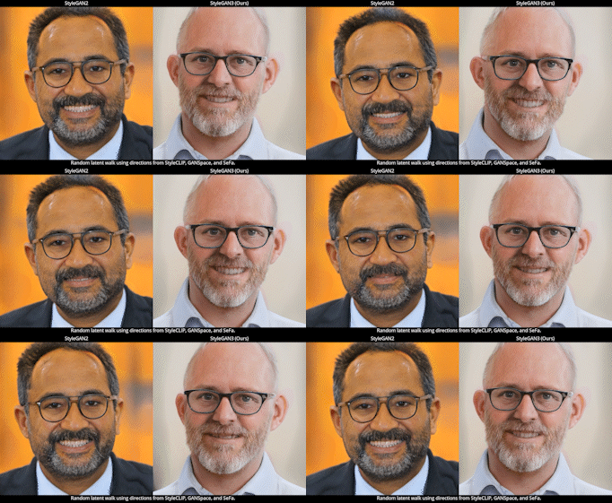
Fig 12. Demo for StyleGAN3. (Image source: https://nvlabs.github.io/stylegan3/)
Video Demo
Colab Demo
Please see deepFake_demo.ipynb in the google drive folder.
Relevant Papers
[1] Siarohin, Aliaksandr, et al. “First Order Motion Model for Image Animation.” Conference and Workshop on Neural Information Processing Systems. 2019.
[2] Choi, Yunjey, et al. “StarGAN v2: Diverse Image Synthesis for Multiple Domains.” IEEE Conference on Computer Vision and Pattern Recognition. 2020.
[3] Choi, Yunjey, et al. “StarGAN: Unified Generative Adversarial Networks for Multi-Domain Image-to-Image Translation.” IEEE Conference on Computer Vision and Pattern Recognition*. 2018.
[4] Zhu, Jun-Yan, et al. “Unpaired Image-to-Image Translation Using Cycle-Consistent Adversarial Networks.” IEEE International Conference on Computer Vision. 2017.
[5] Isola, Phillip, et al. “Image-to-Image Translation with Conditional Adversarial Nets.” IEEE Conference on Computer Vision and Pattern Recognition. 2017.
[6] Mao, Qi, et al. “Mode Seeking Generative Adversarial Networks for Diverse Image Synthesis.” IEEE Conference on Computer Vision and Pattern Recognition. 2019.
[7] Huang, Xun, et al. “Arbitrary Style Transfer in Real-time with Adaptive Instance Normalization.” IEEE International Conference on Computer Vision. 2017.
[8] Huang, Xun, et al. “Multimodal Unsupervised Image-to-Image Translation.” The European Conference on Computer Vision. 2018.
[9] Ren, Yurui, et al. “Deep Image Spatial Transformation for Person Image Generation.” IEEE Conference on Computer Vision and Pattern Recognition. 2020.
[10] Karras, Tero, et al. “A Style-Based Generator Architecture for Generative Adversarial Networks.” IEEE Transactions on Pattern Analysis and Machine Intelligence. 2021.
[11] Zeno, Bassel, et al. “Comparative Review of Cross-Domain Generative Adversarial Networks.” IBIMA conference. 2019.
[12] Karras, Tero, et al. “Alias-Free Generative Adversarial Networks (StyleGAN3).” Conference and Workshop on Neural Information Processing Systems. 2021.