3D Point Cloud understanding is critical for many robotics applications with unstructured environments. Point Cloud Data can be obtained directly (e.g. LIDAR) or indirectly through depth maps (stereo cameras, depth from de-focus, etc.), however efficient merging the information gained from point clouds with 2D image features and textures is an open problem. Graph convolutional networks have the ability to exploit geometric information in the scene that is difficult for 2D based image recognition approaches to reason about and we test how these features can improve classification models.

• Introduction
• Introduction To Graph Neural Networks
• DGCNN
  • EdgeConv
• 2D-3D Fusion
• GeoMat Dataset
• Implementation
  • Feature backbone
  • DeepTen
  • DGCNN
  • 2D-3D Fusion
• Results
  • DeepTen
  • DGCNN
  • Fusion
• Discussion
  • More
  • Reference
  • Code Repository

Introduction

Our project seeks to implement and improve upon graph convolution approaches to 3D point cloud classification and segmentation. We plan to explore the dynamic graph approaches proposed in [1] and [7] which create graphs between each layer with connections between nearby points and uses an asymmetric edge kernel that incorporates relative and absolute vertex locations. This approach contrasts with the typical approach to learning on point clouds which operates directly on sets of points. PointNet [8] is one popular implementation that takes this approach, learning spatial features for each point and using pooling to later perform classification or segmentation.

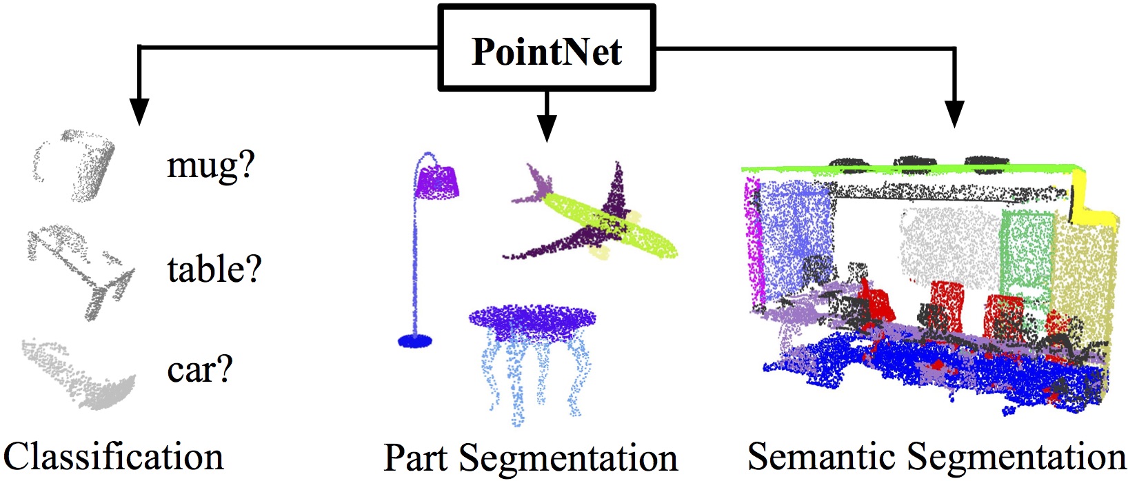
Fig 1. PointNet for learning classification and segmentation tasks on 3D point clouds [8].

Introduction To Graph Neural Networks

Graph Neural Networks, or GNNs, are as the name suggests, neural networks that make sense of graph information. This umbrella term covers graph-level tasks (which our project focuses on), node-level tasks (e.g. predicting the property of a node), and edge-level tasks. GNNs take some input graph \(G = (V, E)\) and transform that graph in some sequence to produce a desired prediction. A basic GNN might look like several layers, each composed of some non-linear function \(f\) (e.g. an MLP) that takes in the current graph \(\mathcal{G}_i\). Depending on the GNN, the graph structure, commonly represented by an adjacency matrix, may stay the same throughout the layers, or change at each layer. The node and/or edge features are progressively transformed by this non-linear mapping and, if the task is graph-level classification, some pooling operation is typically performed to reduce the dimensionality.Depending on the GNN, the graph structure, commonly represented by an adjacency matrix, may stay the same throughout the layers, or change at each layer. For this project, we explored multiple implementations of GNNs, which are explained here.

Fig 2. Convolutions are understood for structured data, but graphs pose a unique problem. [16].

DGCNN

The first network we investigated was a Graph Convolutional Network making use of the EdgeConv convolution operation from [1]. The approach involves modifying the size of the graph at each layer and adding max pooling for each EdgeConv layer. The Dynamic Graph CNN (DGCNN) uses a similar approach, keeping the maximum receptive field, but has the benefit of using fewer parameters for successive layers. The EdgeConv operation is explored more in depth in the following section.

EdgeConv

In order to tackle the problem of maintaining a graph’s permutation invariance while also exploiting the geometric relationship between nodes, Wang et al. proposed a novel differentiable approach called EdgeConv [1]. The method resembles that of typical convolutions in CNNs, where local neighborhood graphs are created for each point and convolution operations are applied on the edges in this neighborhood. Additionally, in contrast to the approaches employed by other graph based networks, these local neighborhoods change after every layer. More specifically, the graph is recomputed after each layer such that the nearest neighbors are now those closest in the feature space. These dynamic graph updates allow the embeddings to be updated globally, and the authors show that this distinction leads to the best results for point cloud classification and segmentation.

Formally, at each layer \(l\), a directed graph \(\mathcal{G^{(l)}} = (\mathcal{V^{(l)}}, \mathcal{E^{(l)}})\) is constructed where each point \(\text{x}_i^{(l)}\) is connected to \(k_l\) other points through edges \((i, j_{i1}) \ldots (i, j_{i k_l})\). To perform this dynamic graph recomputation, the authors compute the pairwise distance between each point in the feature space \(\mathbb{R}^{F}\), and the \(k_l\) nearest neighbors are chosen for each point. With this graph constructed, the output of the actual EdgeConv operation is defined as the aggregation of weighted edge features for each edge in the neighborhood,

Here, \(\square\) represents the chosen aggregation function, such as a summation, max, or average. The edge features \(h_{\Theta}(\text{x}_i, \text{x}_j)\) have learnable parameters \(\Theta\) and map from \(\mathbb{R^F} \times \mathbb{R^F}\) to \(\mathbb{R}^{F'}\). This operation is also shown in Fig 1.

Fig 3. The EdgeConv operation [1].

The choice of \(\square\) and \(h\) can greatly affect the performance of the model. For example, in the case where

the features of the neighboring points are not taken into consideration when computing edge features. The authors choose to use an asymmetric function given by

This choice of edge feature allows for exploiting both global structure as well as local neighborhood shape information. This operator is formulated as

where \(\Theta = (\theta_1, \ldots, \theta_M, \phi_1, \ldots, \phi_M)\) and the aggregation function is chosen as a maximum. This gives a final edge feature representation of

In the original network architecture, shown in Fig 2, four EdgeConv layers are used to find geometric features from the input point clouds. For each of these layers, the number of nearest neighbors \(k\) is chosen as 20. The features from each layer are concatenated and passed through a global max pooling layer followed by two fully connected layers with a dropout of \(p=0.5\). In addition, each layer uses a Leaky ReLU activation with batch normalization. Training is performed using SGD with momentum equal to 0.9, a learning rate of 0.1, and learning rate decay with cosine annealing [1].

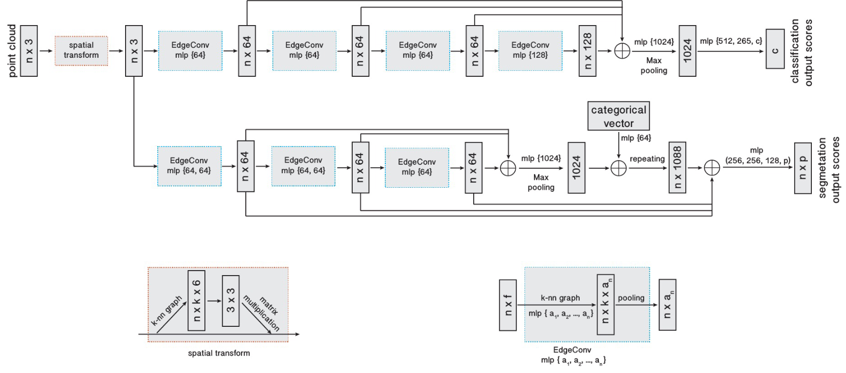
Fig 4. EdgeConv architecture for classification and segmentation [1].

2D-3D Fusion

In addition to DGCNNs, we looked into a second GCN approach inspired by [11] which uses a feature extraction backbone and takes a different approach in using 3D information with its own graph convolution method. The method creates separate graphs for 2D texture and 3D geometric features and uses a fusion technique for combining these features.

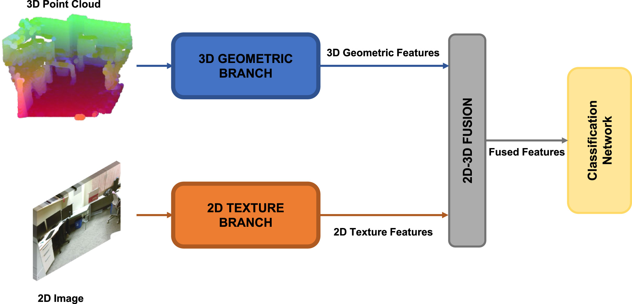
Fig 5. The MUNEGC network high level overview [11].

The feature backbone gives as output 2D texture features, which are then combined with a downsampled point cloud. The 3D features are created using the constructed point cloud and depth information using Attention Graph Convolution (AGC) [10] for both the euclidean and feature neighborhoods. Similar to EdgeConv, AGC has an attention mechanism, but differs in that it only takes edge attributes into account for attention weighting and not the features themselves. This also differs from graph attention networks (GAT) [9] which takes a more common form of attention in which node features as well as the difference between the features and also includes a normalization of the attention coefficient. [11] uses an aggregation of euclidean and feature based AGC called Multi Neighborhood Graph Convolution (MUNEGC).

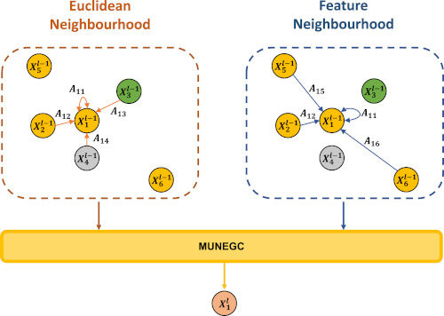
Fig 6. The Multi-Neighborhood Graph Convolution (MUNEGC) operation [11].

The authors of [11] also propose a novel pooling method to be used in conjunction with MUNEGC layers called Nearest Voxel Pooling (NVP). With standard voxel pooling, voxels of resolution \(r_p\) are created over the point cloud in 3D space and the points in each voxel are combined into a centroid with a feature computed through either an average or maximum operation. Nearest Voxel Pooling adds an additional step to address the issue of points in each voxel being closer to neighboring voxel centroids than their own. To do this, every point is grouped into clusters based on their nearest centroid, and any centroid without a corresponding cluster is discarded. Then, based on these groups, new centroids are created based on the position and features of the group.

Fig 7. A comparison of voxel pooling (left) and Nearest Voxel Pooling (right) [11].

GeoMat Dataset

To assess the performance of our DGCNN and fusion networks on point cloud classification, and specifically material prediction, we chose the GeoMat dataset since it includes both RGB and Sparse Depth unlike many other RGB-only material datasets [7]. In addition to the RGBD data, the GeoMat dataset provides camera intrinsics and extrinsics, calculated surface normals, as well as the position of the image patch in the larger image. We use the provided camera intrinsics and sparse depth to project the 2D image points into 3D space and generate a point cloud.

To improve training performance, we pre-process the image by normalizing the RGB channels for each image. Additionally, we augment the 2D image data by performing random flips and rotations. We also normalize the positions of each point to the interval (-1, 1). When extracting 3D geometric features during training, we augmented the 3D data with random dropout of points, rotating about the z-axis between 0 and 180 degrees, and flipping horizontally. We also employ a random 3D cropping method proposed by [11], in which a random point is chosen from the point cloud and a cropping radius is found which includes only a specified fraction \(f\) of the original number of points.

The dataset consists of a total of 19 different materials, with each category consisting of 400 training and 200 testing examples. Training examples from the Cement - Granular, Grass, and Brick classes along with their constructed 3D point clouds are shown in Fig 3.

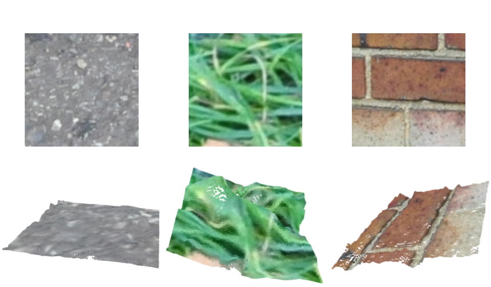
Fig 8. GeoMat training images for Cement, Grass, and Brick, along with constructed point clouds [7].

Implementation

Here we outline the more specific network architectures that were implemented. For training all of these networks, we used an RAdam optimizer with a learning rate of 0.001 and betas of 0.9 and 0.999 as a default. We also used cross-entropy loss with label-smoothing to reduce overconfidence of our models. We used the PyTorch Geometric framework since it provides common operations on graphs and allows for efficient data loading, sampling, and training.

Feature backbone

To generate feature maps for subsequent networks, we adopted the common practice of using a convolutional network as a backbone. Generally, pre-trained networks such as one of the ResNet variations are chosen, and we decided to fine-tune the weights of the last 3 convolution blocks and final classification layers of a \(\verb'convnext_large'\) network [12], chosen for its accuracy and efficiency. The convolutional layers have filter size and depths of \(\verb'192, 384, 768, 1536', \verb'3, 3, 27, 3'\), respectively. The 3rd layer with dimensions \(\verb'512x14x14'\), similar to [13], and use max pooling with kernel sizes 4 and 2 for the first two layers and interpolate the final layer to match the output dimension of the third layer, giving and output feature size of \(\verb'2880x14x14'\). A 1x1 convolution is then used to reduce the feature map channel size to 32.

DeepTen

The baseline image-approach for comparison was based on Deep Texture Encoding Network (DeepTEN) [14], which uses dictionary learning and a residual encoding to learn domain-specific information. This encoding layer was specifically proposed for material recognition tasks and serves as a generalization of encoding schemes such as Fisher Vectors which showed the best performance in [7]. We used ConvNext [12] as our feature backbone, a dictionary with \(\verb'32x128'\) codewords.

DGCNN

We implement 4 separate DGCNN networks, each of which uses MLPs with a leaky ReLu activation slope of -0.2 and dropout of 0.2. While each point cloud has a total of 10000 points, we lower memory consumption for each example by sampling 1000 points from the original. The MLP input used for each EdgeConv layer has double the dimensions of the layer input. The four network architectures are described here:

\(\textit{DG-V1}: k=40\), 3 EdgeConv layers \(\verb'[6, 64],[128,128],[256,256]'\) and 2 MLP layers \(\verb'[448, 1024],[1024, 512, 256, 19]'\).

\(\textit{DG-V2}: k=20\), 4 EdgeConv layers \(\verb'[6, 64],[128,64],[128, 128],[256,256]'\) and 2 MLP layers \(\verb'[512, 1024],[1024, 512, 256, 19]'\).

\(\textit{DG-V3}\): 1 2D Conv for the feature backbone: \(\verb'[1344, 128]'\), 4 EdgeConv layers \(\verb'[268, 64],[128,128],[256,256]'\) and 2 MLP layers \(\verb'[576, 1024],[1024, 512, 256, 19]'\).

\(\textit{DG-V4}\): 1 2D Conv for the feature backbone: \(\verb'[64]'\), 4 EdgeConv layers \(\verb'[6, 64],[128,64]'\) and 2 MLP layers \(\verb'[192, 1024],[1024, 512, 256, 19]'\).

We see a simplified version of \(\textit{DG-V4}\) below:

class DGCNN(torch.nn.Module):
    def __init__(self, out_channels, k=20, aggr="max", dropout=0.8):
        super().__init__()
        self.conv1 = DynamicEdgeConv(MLP([2 * (3 + 3), 64], act="LeakyReLU", act_kwargs={"negative_slope": 0.2}, dropout=dropout), k, aggr)
        self.conv2 = DynamicEdgeConv(MLP([2 * 64, 64], act="LeakyReLU", act_kwargs={"negative_slope": 0.2}, dropout=dropout), k, aggr)
        self.fc1 = MLP([64 + 64, 1024], act="LeakyReLU", act_kwargs={"negative_slope": 0.2}, dropout=dropout)
        self.fc2 = MLP([1024 + 2304, 512, 256, out_channels], dropout=dropout)

        self.img_model = timm.create_model("convnext_base", num_classes=2, drop_path_rate=dropout).cuda()
        self.img_model.eval() # Don't fine-tune layers to reduce computation
        self.filter_conv = nn.Conv2d(1920, 64, 1)  # reduce filter size

    def forward(self, data):
        pos, x, batch = (data.pos.cuda(), data.x.cuda(), data.batch.cuda())
        features = self.img_model.get_features_concat(data.image.cuda().permute(0, 3, 1, 2).float())
        features = self.filter_conv(features)
        x1 = self.conv1(torch.cat((pos, x), dim=1).float(), batch)
        x2 = self.conv2(x1, batch)
        out = self.fc1(torch.cat((x1, x2), dim=1))
        out = global_max_pool(out, batch)
        out = self.fc2(torch.cat((out, features.reshape(features.shape[0], -1)), dim=1))
        return F.log_softmax(out, dim=1)

We also show the implementation of the EdgeConv operator (seen above as DynamicEdgeConv). The core of the code is the forward method where the KNN function is called and the message function where x_i and x_i - x_j are passed through the specified nonlinear function (in our case an MLP):

class DynamicEdgeConv(MessagePassing):
    ...
    def forward(self, x, batch):
        if isinstance(x, Tensor):
            x: PairTensor = (x, x)

        ...

        b = (None, None)
        if isinstance(batch, Tensor):
            b = (batch, batch)
        elif isinstance(batch, tuple):
            assert batch is not None
            b = (batch[0], batch[1])

        edge_index = knn(x[0], x[1], self.k, b[0], b[1]).flip([0])

        # propagate_type: (x: PairTensor)
        return self.propagate(edge_index, x=x, size=None)

    def message(self, x_i, x_j):
        return self.nn(torch.cat([x_i, x_j - x_i], dim=-1))

2D-3D Fusion

The fusion approach inspired by [11] uses 3 separately trained networks. The first two are used to extract 2D texture and 3D geometric feature graphs from the input data. After these features are fused, the third network performs classification.

2D Features

To extract the 2D texture features graph, we use the our ConvNext backbone along with 2D average pooling to match a final feature size of \((\verb'14x14')\).

3D Features

To extract the 3D geometric features graph, we use a GCN with MUNEGC and NVP layers from [11]. The architecture uses 4 blocks of graph convolution (MUNEGC) along with batch normalization, ReLU nonlinearity, and pooling (NVP). There is also one additional block without the NVP layer, the output of which is then passed to a global average pooling, dropout, and fully connected layer for classification. The 5 MUNEGC layers have feature output sizes of \(\verb'16, 16, 32, 64, 128'\), and the 4 NVP layers have a voxel resolution of \(\verb'0.05, 0.08, 0.12, 0.24'\), respectively. The classification head uses a dropout of 0.2, and the fully connected layer has output size 19. Once the network is trained, 3D geometric feature graphs are taken as the output of the final MUNEGC layer. Partial implementation of the AGC operator used for MUNEGC is shown below, courtesy of [10].

class AGC(torch.nn.Module):
    ...
    def forward(self, x, edge_index, edge_attr):
        x = x.unsqueeze(-1) if x.dim() == 1 else x
        edge_attr = edge_attr.unsqueeze(-1) if edge_attr.dim() == 1 else edge_attr

        i, j = (0, 1) if self.flow == "target_to_source" else (1, 0)

        src_indx = edge_index[j]
        target_indx = edge_index[i]

        # weights computation
        out = self._wg(edge_attr)
        out = out.view(-1, self.in_channels, self.out_channels)

        N, C = x.size()

        feat = x[src_indx]

        out = torch.matmul(feat.unsqueeze(1), out).squeeze(1)
        out = scatter(out, target_indx, dim=0, dim_size=N, reduce=self.aggr)

        if self.bias is not None:
            out = out + self.bias

        return out

Fusion

To fuse the 2D texture and 3D geometric feature graphs obtained from the previous two networks, we implemented the fusion approach from [11]. The 2D features with dimension \(\verb'1920'\) are first projected to 3D space, then both the 2D and 3D (size \(\verb'128'\)) features are passed through a ReLU nonlinearity along with 1x1 convolution to give both features a size of \(\verb'512'\). A modified version of NVP is then used, in which for each centroid, the newly assigned feature is given as the concatenation of the separately calculated 2D and 3D feature averages in each group, as opposed to the average of all the features together. This is shown in Fig. 9. Once the features are fused with a voxel resolution of 0.24, they are used with a standard classification network using batch normalization, ReLU nonlinearity, global average pooling, dropout, and a fully connected layer. The chosen dropout is 0.5, and the final output size is 19. The fusion step is shown below.

class MultiModalGroupFusion(torch.nn.Module):
    ...
    def forward(self, b1, b2):
        pos = torch.cat([b1.pos, b2.pos], 0)
        batch = torch.cat([b1.batch, b2.batch], 0)

        batch, sorted_indx = torch.sort(batch)
        inv_indx = torch.argsort(sorted_indx)
        pos = pos[sorted_indx, :]

        start = pos.min(dim=0)[0] - self.pool_rad * 0.5
        end = pos.max(dim=0)[0] + self.pool_rad * 0.5

        cluster = torch_geometric.nn.voxel_grid(pos, self.pool_rad, batch, start=start, end=end)
        cluster, perm = consecutive_cluster(cluster)

        superpoint = scatter(pos, cluster, dim=0, reduce="mean")
        new_batch = batch[perm]

        cluster = nearest(pos, superpoint, batch, new_batch)

        cluster, perm = consecutive_cluster(cluster)

        pos = scatter(pos, cluster, dim=0, reduce="mean")
        branch_mask = torch.zeros(batch.size(0)).bool()
        branch_mask[0 : b1.batch.size(0)] = 1

        cluster = cluster[inv_indx]

        nVoxels = len(cluster.unique())

        x_b1 = torch.ones(nVoxels, b1.x.shape[1], device=b1.x.device)
        x_b2 = torch.ones(nVoxels, b2.x.shape[1], device=b2.x.device)

        x_b1 = scatter(b1.x, cluster[branch_mask], dim=0, out=x_b1, reduce="mean")
        x_b2 = scatter(b2.x, cluster[~branch_mask], dim=0, out=x_b2, reduce="mean")

        x = torch.cat([x_b1, x_b2], 1)
        ...

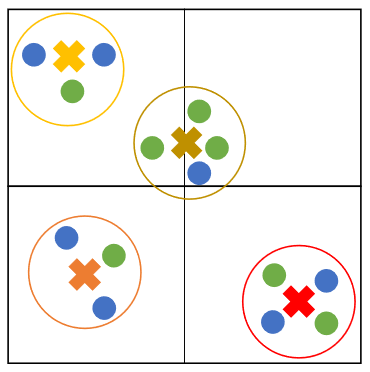
Fig 9. Fusing 2D (blue) and 3D (green) features with NVP [11].

Results

The results of our experiments are shared here. Training curves are shown in Fig. 10, 11 and test set results are shown in Fig. 12.

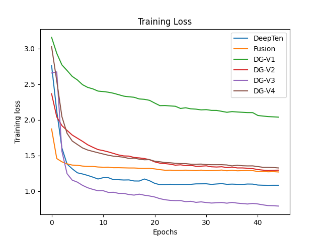
Fig 10. Training loss.

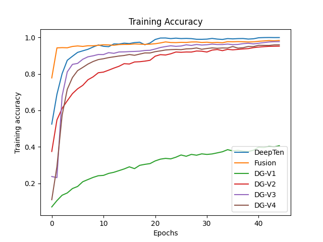
Fig 11. Training accuracy.

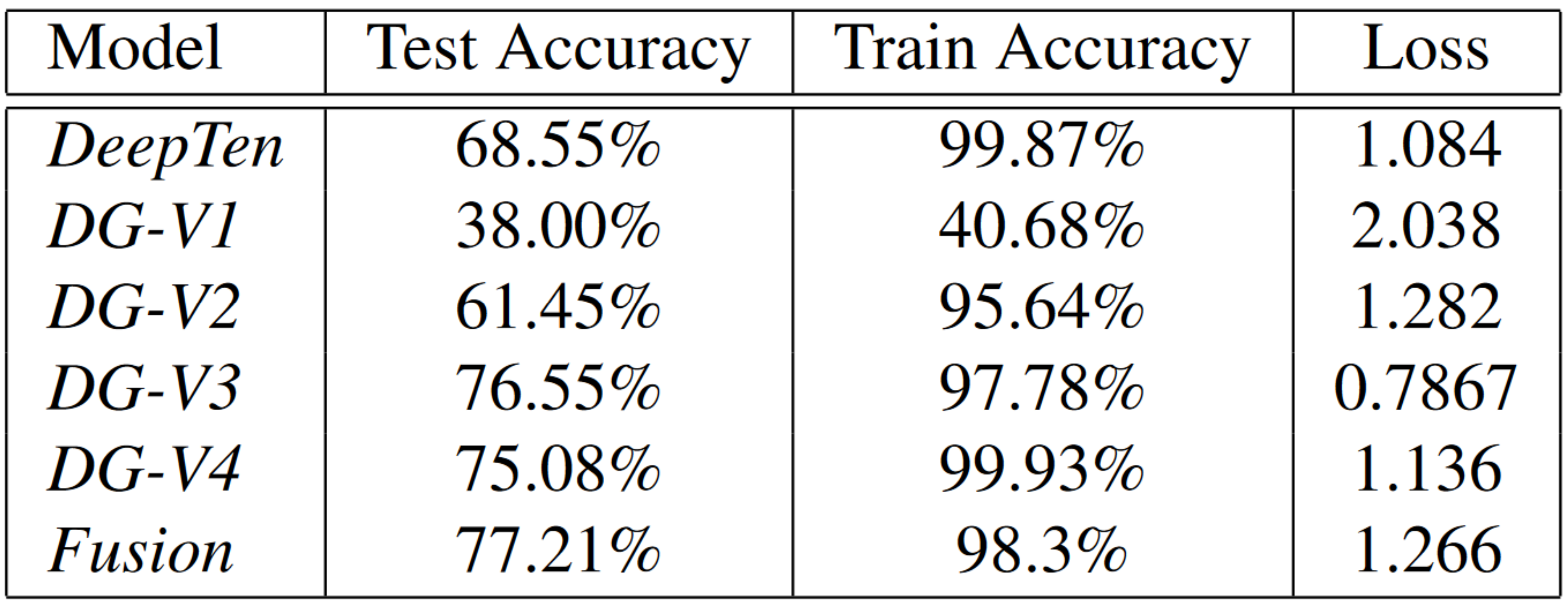
Fig 12. Test results. Accuracy taken as best from all epochs, training loss and accuracy after 50 epochs.

DeepTen

Our baseline, 2D RGB data only network using the ConvNext backbone, encoding layer, and fully connected layer achieves \(\textbf{68.55%}\) test accuracy.

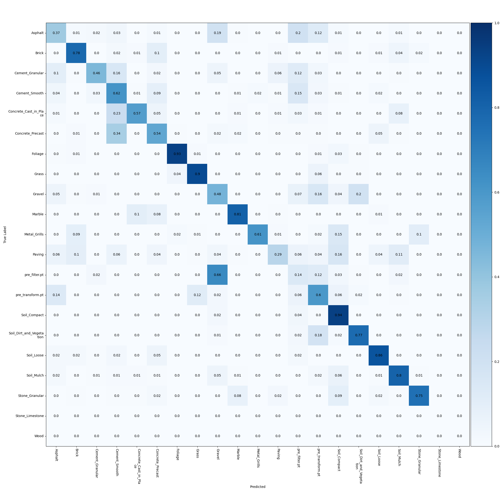
Fig 13. Confusion matrix for DeepTen network.

DGCNN

Our first DGCNN implementation using exclusively 3D depth data achieves only \(\textbf{38.00%}\) test accuracy \((\textit{DG-V1})\). We notice significant improvement after adding RGB information as features for each node, giving a test accuracy of \(\textbf{61.45%}\) \((\textit{DG-V2})\). The best performing DGCNN network that we implemented uses the ConvNext backbone as well as both RGB and depth data for each node used with the four EdgeConv and two fully layers. These additions give a accuracy of \(\textbf{76.55%}\) on the test set \((\textit{DG-V3})\).

For our fourth DGCNN implementation, we use a lightweight network using only 2 EdgeConv and 2 fully connected layers, along with a lighter ConvNext backbone. The lightweight model uses a total of 89 million parameters, compared to the 198 million parameters used in the full scale version \(\textit{DG-V3}\). 2D image features are not passed to the EdgeConv layers, only the fully connected layers, which significantly reduced computation. This lighter model had a test accuracy of \(\textbf{75.08%}\) \((\textit{DG-V4})\). This verifies our thinking in that graph convolution is not as appropriate for processing the extracted image features which have less of a meaningful graph structure, as opposed to the unprocessed pixel-wise data.

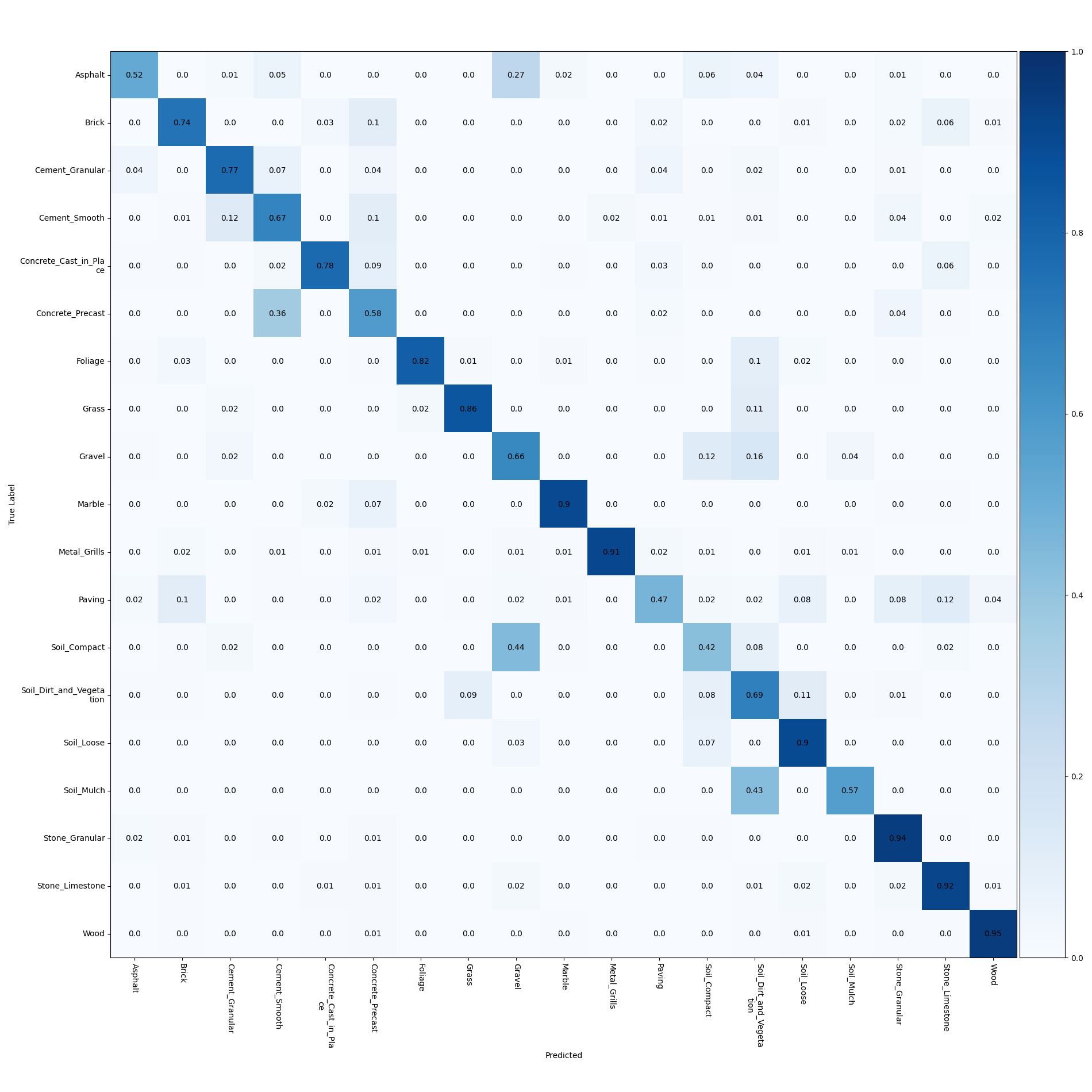
Fig 14. Confusion matrix for DG-V3 network.

Fusion

The classification network using the fused 2D texture and 3D geometric features achieved a test accuracy of \(\textbf{77.21%}\). This is over 3% higher than the best result achieved by the group who created the GeoMat dataset, 73.84% [7].

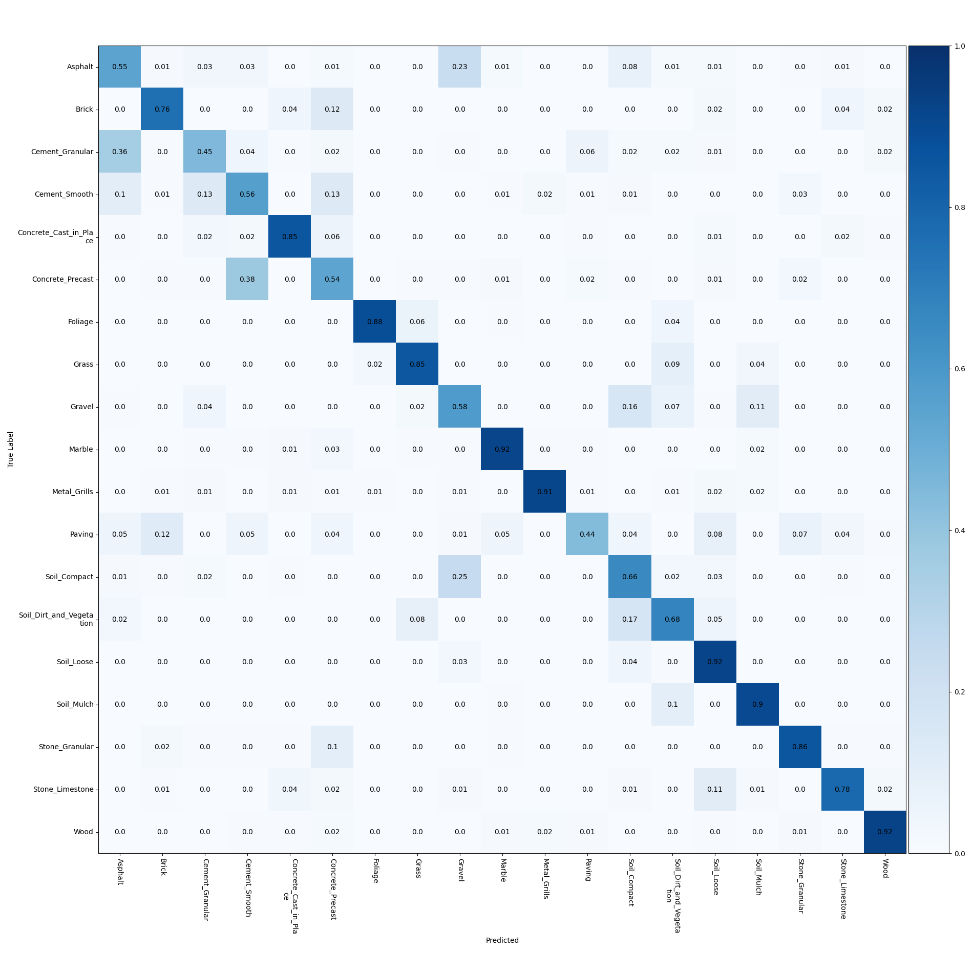
Fig 15. Confusion matrix for fusion network.

Discussion

For the results above, we notice that using only geometric features gives below 40% test accuracy, whereas the approaches that also make use of the RGB data all achieve well over 60% test accuracy. This is most likely due to the resolution of the given depth data. Since the depth map is relatively sparse, many of the materials which have similar geometry would have similar depth maps. This is also confirmed by observing the confusion matrix for the networks using both 2D and 3D data in Figs. 14 and 15. Many of the errors occur between materials such as paving, cement, asphalt, or the concrete classes, all of which would have similar geometries. To address this issue, we could also make use of the provided contextual depth data which gives information about the rest of the scene from which the patch is taken. This could give similar improvements as shown in using contextual encoding of image features in semantic segmentation approaches with RGB data [15].

However, even if the depth data is imperfect, we do notice significant improvement when incorporating the 3D data alongside the RGB image when compared to our RGB only baseline. For each DGCNN version, we were able to achieve these improvements by adding extracted image features, increase the number of neighbors \(k\), and fine-tuning the ConvNext backbone weights.

Our best results come from the fusion network making use of MUNEGC, giving a slightly higher accuracy (0.66%) compared to our best DGCNN approach. While these approaches have many differences, we refrain from making too many direct comparisons. However, both approaches greatly benefit from passing image features to the fully connected layers following the graph convolutions. The fusion network uses two completely separated branches for the 2D and 3D features, and the best performing DGCNN networks ( \(\textit{DG-V3, DG-V4}\)) use a skip connection over the graph convolution layers. The importance of this is clearly seen in the significant performance difference between the DGCNN networks which do and don’t (\(\textit{DG-V2}\)) use the approach.

More

Here’s a link to our Github repository where our work can be found for those interested.

Also, our video spotlight is below.

Reference

[1] Y. Wang, Y. Sun, Z. Liu, S. E. Sarma, M. M. Bronstein, and J. M. Solomon, “Dynamic graph CNN for learning on point clouds,” ACM Transactions on Graphics, vol. 38, no. 5, pp. 1–12, 2019.

[2] X. Wei, R. Yu, and J. Sun, “View-GCN: View-based graph convolutional network for 3D shape analysis,” 2020 IEEE/CVF Conference on Computer Vision and Pattern Recognition (CVPR), 2020.

[3] Q. Xu, X. Sun, C.-Y. Wu, P. Wang, and U. Neumann, “Grid-GCN for fast and Scalable Point Cloud Learning,” 2020 IEEE/CVF Conference on Computer Vision and Pattern Recognition (CVPR), 2020.

[4] Y. Chai, P. Sun, J. Ngiam, W. Wang, B. Caine, V. Vasudevan, X. Zhang, and D. Anguelov, “To the point: Efficient 3D object detection in the range image with graph convolution kernels,” 2021 IEEE/CVF Conference on Computer Vision and Pattern Recognition (CVPR), 2021.

[5] H. Haotian, F. Wang and H. Le. “VA-GCN: A Vector Attention Graph Convolution Network for learning on Point Clouds.” ArXiv abs/2106.00227 2021.

[6] L. Chen and Q. Zhang, “DDGCN: Graph convolution network based on direction and distance for point cloud learning,” The Visual Computer, 2022.

[7] J. DeGol, M. Golparvar-Fard, and D. Hoiem, “Geometry-Informed Material Recognition,” 2016 IEEE/CVF Conference on Computer Vision and Pattern Recognition (CVPR), 2016.

[8] R. Q. Charles, H. Su, M. Kaichun, and L. J. Guibas, “PointNet: Deep learning on point sets for 3D classification and segmentation,” in Proc. IEEE CVPR, Jul. 2017

[9] P. Velickovic, G. Cucurull, A. Casanova, A. Romero, P. Lio, and Y. Bengio. Graph attention networks. arXiv preprint arXiv:1710.10903, 2017.

[10] A. Mosella-Montoro and J. Ruiz-Hidalgo. Residual attention graph convolutional network for geometric 3d scene classification. In Proceedings of the IEEE/CVF International Conference on Computer Vision Workshops, pages 0–0, 2019.

[11] A. Mosella-Montoro and J. Ruiz-Hidalgo. 2d–3d geometric fusion network using multi-neighbourhood graph convolution for rgb-d indoor scene classification. Information Fusion, 76:46–54, 2021.

[12] Z. Liu, H. Mao, C.-Y. Wu, C. Feichtenhofer, T. Darrell, and S. Xie. A convnet for the 2020s. arXiv preprint arXiv:2201.03545, 2022.

[13] S. Casas, A. Sadat, and R. Urtasun. Mp3: A unified model to map, perceive, predict and plan. In Proceedings of the IEEE/CVF Conference on Computer Vision and Pattern Recognition, pages 14403–14412, 2021.

[14] H. Zhang, J. Xue, and K. Dana. Deep ten: Texture encoding network. In Proceedings of the IEEE conference on computer vision and pattern recognition, pages 708–717, 2017.

[15] H. Zhang, K. Dana, J. Shi, Z. Zhang, X. Wang, A. Tyagi, and A. Agrawal. Context encoding for semantic segmentation. In Proceedings of the IEEE conference on Computer Vision and Pattern Recognition, pages 7151–7160, 2018.

[16] Daigavane, et al., “Understanding Convolutions on Graphs”, Distill, 2021.

Code Repository

[1] Dynamic Graph CNN for Learning on Point Clouds

[2] Pytorch code for view-GCN

[3] Grid-GCN for Fast and Scalable Point Cloud Learning

[4] ModelNet40 Dataset