Pose Estimation

Pose estimation is the use of machine learning to estimate the pose of a person or animal from an image or a video by examining the spatial locations of key body joints. Our project will consist of two main parts: (1) this article, detailing pose estimation background and modeling techniques (2) an interative Google Colaboratory document demonstrating pose estimation in action.

• Spotlight Presentation
• Background
  • Instance Segmentation
  • Top-down vs. Bottom-up methods
  • Types of Human Body Modeling
  • Challenges
  • Datasets
• Models
  • OpenPose
  • Mask R-CNN
• Innovation
  • Residual Steps Network (RSN)
• Applications
  • Google Colaboratory Demo
• Paper References
• Learning References

Spotlight Presentation

Below, you can find a video overview of the below article and a walkthrough of how to use our Google Colaboratory demo.

Background

Just over a decade ago, the task of pose estimation seemed near impossible computationally. However, with recent advances in GPU, TPU, and other computing spaces, applications incorporating pose estimation are becoming commonplace.

In this article, we will discuss the background terminology, modeling techniques, and applications of pose estimation.

First, we will discuss key terminologies, challenges, and datasets related to pose estimation that will give us the necessary context for understanding the modeling techniques discussed later.

Instance Segmentation

Instance segmentation is the process of classifying individual objects and then localizing each of them with a bounding box. This is different from semantic segmentation, which classifies an image pixel by pixel and treats all pixels in the same class as one object.

With a single-object image, the only tasks necessary are classifying, which is giving a class to the main object, and localizing, which is finding the object’s bounding box. With multiple-object images, object detection is required to carry this task out for each object in the image and differentiate between different objects.

Top-down vs. Bottom-up methods

All pose estimation models can be grouped into bottom-up and top-down methods.

• Top-down methods detect a person first and then estimate body joints within the detected bounding boxes.
• Bottom-up methods estimate each body joint first and then group them to form a unique pose.

Types of Human Body Modeling

• Kinematic model
  • Also called skeleton-based model
  • Used for 2D and 3D applications
  • Used to capture the relations between different body parts
• Planar model
  • Also called contour-based model
  • Used for 2D applications
  • Used to represent the appearance and shape of a human body
  • Body parts are represented by multiple rectangles approximating the human body contours
• Volumetric model
  • Used for 3D applications
  • Used to represent the relations between different body parts and the shape of a human body (combination of Kinematic and Planar models)

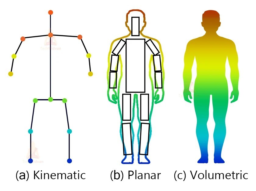
Fig 1. The three types of human body models.

Challenges

Many factors make human pose estimation difficult, including abnormal viewing angles, different background contexts, overlapping body parts, and different clothing shapes. The pose estimation method must also account for real-world variations such as lighting and weather. In addition, small joints can be difficult to detect.

Datasets

The MS COCO dataset is the most popular dataset for human pose estimation. It features 17 different classes, known as keypoints. The classes are listed below. Each keypoint is annotated with three numbers (x,y,v), where x and y mark the coordinates and v indicates if the keypoint is visible.

"nose", "left_eye", "right_eye", "left_ear", "right_ear", "left_shoulder", "right_shoulder", 
"left_elbow", "right_elbow", "left_wrist", "right_wrist", "left_hip", "right_hip", "left_knee",
"right_knee", "left_ankle", "right_ankle"

Models

Now that we have some intuition behind the background and challenges of pose estimation, let’s dive into some of the models that address this task.

We will discuss OpenPose in depth as it was one of the breakthrough models in pose estimation and is very well documented. We will also briefly cover Mask R-CNN because it was discussed in class, and we would like to explain its application to pose estimation.

OpenPose

While OpenPose [1] may not be the gold standard for pose estimation today (see “Innovation” section), it was the first real-time multi-person detection system, and it was the winner of COCO KeyPoint Detection Challenge in 2016. It is important to understand the inner workings of OpenPose as this will provide intuition for understanding successive models and intuition for how to tackle the pose estimation task.

OpenPose is a bottom-up model, and it follows the pipeline below.

Fig 2. OpenPose Pipeline.

• (a): A color input image of size \(w×h\). A feedforward network processes this input image to simultaneously produce…
• (b): A set of 2D Part Confidence Maps (CMs) of body part locations
• (c): A set of 2D vector fields of part affinities, or Part Affinity Fields (PAFs), which encode the degree of association between body parts
• (d): The CMs and the PAFs are parsed by greedy inference, and bipartite matching is performed to associate body part candidates.
• (e): Output the 2D keypoints for all people in the image.

Now, that we have a general idea of the OpenPose pipeline, let’s dive into the technical details and examine the reasoning behind this architecture.

As previously mentioned, the first step is a feedforward network predicts a set of Confidence Maps S and a set of Part Affinity Fields L. The set \(S = (S_1, S_2, …, S_J)\) has \(J\) confidence maps, one per body part location, where \(S_j ∈ R^{w×h}, j ∈ \{1 … J\}\). The set \(L = (L_1, L_2, …, L_C)\) has \(C\) vector fields, one per limb, where \(L_c ∈ R^{w×h×2}, c ∈ \{1 … C\}\). Each image location in \(L_c\) encodes a 2D vector.

The baseline arhitecture is seen in the image below.

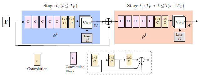
Fig 3. OpenPose Network Architecture.

It works by iteratively predicting part affinity fields that encode part-to-part association, shown in blue, and detection confidence maps, shown in beige. Predicions are refined over successive stages, \(t ∈ {1, …, T}\), with supervision at each stage.

In the above image, the unit titled as \(Convolution \: Block\) consists of 3 consecutive 3x3 kernels. The output of each one of the 3 convolutional kernels is concatenated, tripling the number of non-linear layers compared to not using concatenation. This allows the the network to catpure both low level and high level features.

As a note, for the input to the first stage, feature extraction is performed by VGG-19 to produce the set of feature maps \(F\). For this stage, the blue region in Fig 3. produces a set of PAFs, \(L^1 = \phi^1(F)\), where \(L^1\) refers to the PAFs at Stage 1 and \(\phi^1\) refers to the CNN at Stage 1. For each subsequent stage, the original image features \(F\) and the PAFs from the previous stage are concatenated to produce the new PAFs. This is summarized by the equation below,

where \(\phi^t\) refers to the CNN at Stage \(t\) and \(T_P\) refers to the number of total PAF stages. After \(T_P\) iterations, a similar process is repeated for producing confidence maps, beige region in Fig. 3. This is summarized by the equations below,

where \(\rho^t\) refers to the CNN at Stage \(t\) and \(T_C^p\) refers to the number of total CM stages.

We can see the refinement of our predictions increase across stages in the toy example below. Initially, there is confusion whether this is a left or right body part in the early stages, but this distinction is refined in later stages.

Fig 3. PAFs of right forearm across stages.

Now, let us delve into the loss functions for our architecture. From Fig 3., we see a loss function \(f^{t}_L\) applied on the PAFs and a loss function \(f^{t}_S\) applied on the CMs. The loss functions use an L2 loss between the predictions and groundtruth maps and fields. Additionally, we apply a weight to our loss functions to address a dataset issue where all people are not always completely labeled. More formally, the loss function of the PAF branch at stage \(t_i\) and the loss function of the CM branch at stage \(t_k\) are:

where \(L^*_c\) is the groundtruth PAF, \(S^*_j\) is the groundtruth CM, and \(W\) is a binary mask with \(W(p) = 0\) when the annotation is missing at pixel \(p\). During training, the mask prevents penalizing true positive predictions. To address the vanishing gradient problem, OpenPose replenishes the gradient periodically. Summarizing the previous two loss functions, the overall objective function \(f\) can then be written as:

Below, you can see some of the test results that OpenPose had on the COCO test-dev dataset.

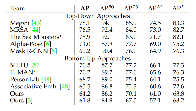
Fig 3. OpenPose performance on COCO test-dev dataset.

This concludes our technical discussion of OpenPose. Below, you can find additional information on Confidence Maps and Part Affinity Fields for further reading.

OpenPose Confidence Maps

The confidence maps are a measure of the likelihood of a given body part being located at any given pixel. For example, the confidence map of the right knee should be 0 in every grid area that a right knee is not present. There is one set, S, for each body part, adding up to J sets that make up the confidence maps.

However, confidence maps are not as crucial to accuracy as Part Affinity Fields are, and some models omit them entirely since they tend to not increase the Average Precision or Average Recall.

OpenPose Part Affinity Fields

The Part Affinity Fields connect parts of the body that belong to the same person. For example, if an area is classified as “left_elbow” and another area is classified as “left_wrist,” the PAF tells you how likely it is that those two body parts belong to the same person. This proves helpful when images contain multiple people overlapping or standing close to each other, like in crowd situations.

The exact methods of determining this association strength can be done multiple ways, such as:

• A k-partite graph
• A bi-partite graph with a greedy algorithm
• A tree structure
• Body part classification

Mask R-CNN

Mask R-CNN is a popular tool for segmenting an image by its pixels (semantically) or by its image objects (instantially). As such, it is not difficult to apply Mask R-CNN to pose estimation.

Once a CNN extracts features from the image, a Region Proposal Network generates bounding box candidates where objects could be. Another layer reduces the features to those of similar size, then runs them in parallel to get segmentation mask proposals. These are used to create binary masks of where an object is and is not present in the image. Finally, keypoints are extracted by segmenting, then combined with the person locations to get a human skeleton for each figure.

This is similar to a top-down approach, except that the person detection step and the body joint estimation step happen in parallel.

As we discussed in class, what is cool about the Mask R-CNN is from the base Mask R-CNN, we can apply different per-region heads that allow us to perform various downstream tasks. Obviously, in our case, we apply a “head” that allows for keypoint prediction.

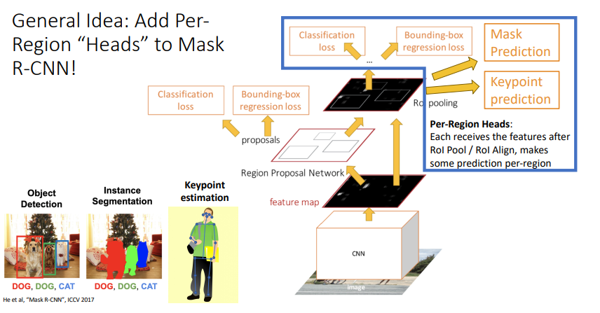
Fig 4. Diagram of Mask R-CNN and keypoint prediction head applied.

Innovation

Residual Steps Network (RSN)

While this is not our improvement, we wanted to highlight one of the more modern architectures for pose estimation as we felt it was important to discuss innovations in the field. The RSN model [3] was the winner of the COCO KeyPoint Detection Challenge in 2019.

RSN [3] was created with the goal of having the accuracy of the DenseNet model without the huge network capacity requirements. It incorporates ideas from ResNet, and it uses a Residual Steps Block, or RSB, to fuse features with element-wise sum operations rather than concatenation.

Below, we have included the source code of the RSN class to help readers get an idea of how the creators went about having the RSN aggregate features in order to learn delicate local representations within the image in order to obtain precise keypoint locations.

class RSN(nn.Module):
    
    def __init__(self, cfg, run_efficient=False, **kwargs):
        super(RSN, self).__init__()
        self.top = ResNet_top()
        self.stage_num = cfg.MODEL.STAGE_NUM
        self.output_chl_num = cfg.DATASET.KEYPOINT.NUM
        self.output_shape = cfg.OUTPUT_SHAPE
        self.upsample_chl_num = cfg.MODEL.UPSAMPLE_CHANNEL_NUM
        self.ohkm = cfg.LOSS.OHKM
        self.topk = cfg.LOSS.TOPK
        self.ctf = cfg.LOSS.COARSE_TO_FINE
        self.mspn_modules = list() 
        for i in range(self.stage_num):
            if i == 0:
                has_skip = False
            else:
                has_skip = True
            if i != self.stage_num - 1:
                gen_skip = True
                gen_cross_conv = True
            else:
                gen_skip = False 
                gen_cross_conv = False 
            self.mspn_modules.append(
                    Single_stage_module(
                        self.output_chl_num, self.output_shape,
                        has_skip=has_skip, gen_skip=gen_skip,
                        gen_cross_conv=gen_cross_conv,
                        chl_num=self.upsample_chl_num,
                        efficient=run_efficient,
                        **kwargs
                        )
                    )
            setattr(self, 'stage%d' % i, self.mspn_modules[i])

    def _calculate_loss(self, outputs, valids, labels):
        # outputs: stg1 -> stg2 -> ... , res1: bottom -> up
        # valids: (n, 17, 1), labels: (n, 5, 17, h, h)
        loss1 = JointsL2Loss()
        if self.ohkm:
            loss2 = JointsL2Loss(has_ohkm=self.ohkm, topk=self.topk)
        
        loss = 0
        for i in range(self.stage_num):
            for j in range(4):
                ind = j
                if i == self.stage_num - 1 and self.ctf:
                    ind += 1 
                tmp_labels = labels[:, ind, :, :, :]

                if j == 3 and self.ohkm:
                    tmp_loss = loss2(outputs[i][j], valids, tmp_labels)
                else:
                    tmp_loss = loss1(outputs[i][j], valids, tmp_labels)

                if j < 3:
                    tmp_loss = tmp_loss / 4

                loss += tmp_loss

        return dict(total_loss=loss)
        
    def forward(self, imgs, valids=None, labels=None):
        x = self.top(imgs)
        skip1 = None
        skip2 = None
        outputs = list()
        for i in range(self.stage_num):
            res, skip1, skip2, x = eval('self.stage' + str(i))(x, skip1, skip2)
            outputs.append(res)

        if valids is None and labels is None:
            return outputs[-1][-1]
        else:
            return self._calculate_loss(outputs, valids, labels)

Below, you can see some of the test results that RSN had on the COCO test-dev and COCO test-challenge datasets.

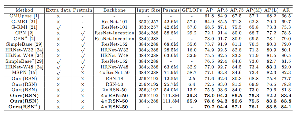
Fig 3. RSN performance on COCO test-dev dataset. ”” means using ensembled models. Pretrain = pretrain the backbone on the ImageNet classification task.*

Fig 3. RSN performance on COCO test-challenge dataset. ”” means using ensembled models. Pretrain = pretrain the backbone on the ImageNet classification task.*

As you can see from these results, RSN has a considerable performance improvement compared to OpenPose.

Applications

Pose estimation has applications in a number of areas.

• Human Health and Performance
  • Performing motor assessments on patients remotely, especially in pediatrics
    • this can detect disorders that cause atypical development in children
  • Evaluating athletic performances
  • Analyzing gait, especially for people having a stroke or with dementia
• Driver Safety
  • Identifying driver drowsiness or distraction with head pose estimation
  • Predicting cyclists’ behavior by their hand signs
  • Vehicle pose estimation
• Entertainment
  • Tracking hand poses instead of having players hold controllers in VR
  • Producing deepfakes of dancing, like Sway from Humen.Ai
  • Snapchat’s Lens Studio, a form of augmented reality

Google Colaboratory Demo

Below, please see the Google Colaboratory demo we have put together to show pose estimation in action! You will be able to upload your own YouTube video and observe pose estimation applied to it.

Demo

Paper References

[1] Cao, Zhe, et al. “OpenPose: Realtime Multi-Person 2D Pose Estimation using Part Affinity Fields” arXiv preprint arXiv:1812.08008 (2019).
[Paper] [Code]

[2] Luo, Zhengyi, et al. “Dynamics-Regulated Kinematic Policy for Egocentric Pose Estimation” arXiv preprint arXiv:2106.05969 (2021).
[Paper] [Code]

[3] Cai, Yuanhao, et al. “Learning Delicate Local Representations for Multi-Person Pose Estimation” arXiv preprint arXiv:2003.04030 (2020).
[Paper] [Code]

Learning References

[4] Odemakinde, Elisha. “Human Pose Estimation with Deep Learning – Ultimate Overview in 2022.” Viso.ai, https://viso.ai/deep-learning/pose-estimation-ultimate-overview/. Accessed 16 Mar. 2022.

[5] Research Team. “An Overview of Human Pose Estimation with Deep Learning.” BeyondMinds, https://beyondminds.ai/blog/an-overview-of-human-pose-estimation-with-deep-learning/. Accessed 16 Mar. 2022.