Behaviour prediction in dynamic, multi-agent systems is an important problem in the context of self-driving cars. In this blog, we will investigate a few different approaches to tackling this multifaceted problem and reproduce the work of Gao, Jiyang et al. by implementing VectorNet in PyTorch.

Introduction

Self-driving is one of the biggest applications of Computer Vision in industry. Naturally, being able to predict the trajectory of an autonomous vehicle is paramount to the success of self-driving. Our project will be an extension of VectorNet: Encoding HD Maps and Agent Dynamics from Vectorized Representation, which is a hierachical graph neural network architecture that first exploits the spatial locality of individual road components represented by vectors and then models the high-order interactions among all components. Research on trajectory prediction is not limited to the self-driving domain, however, Social LSTM: Human Trajectory Prediction in Crowded Spaces and Social GAN: Socially Acceptable Trajectories with Generative Adversarial Networks are more generic examples of work related to multi-agents interaction forecasting which we will also explore in this project. In particular, if possible, we will attempt to extend the work on human trajectory prediction in crowded spaces to simulate the effect that social distancing due to COVID-19 has on the trajectories. We may be able to do this by exploring ways of adding a factor to create a form of ‘repulsion’ between the agents.

Paper 1: VectorNet - Encoding HD Maps and Agent Dynamics From Vectorized Representation

Introduction

Predicting the behaviour of others on the road is difficult: often, a holistic understanding of a scene and its context is required, including the width of road lanes, four-way intersection rules, traffic lights, and signs. Recent learning-based approaches to tackling behaviour prediction require building a representation to encode the map and trajectory information, often in the form of High Definition (HD) maps. These HD maps are rendered as color-coded attributes (Fig 1, left), which encode scene context information, such as traffic signs, lanes, and road boundaries, with ConvNets. These approaches have a few drawbacks. First and foremost, utilizing ConvNets to encode scene context information requires a lot of compute and time. In addition, processing maps as imagery makes it challenging to model long-range geometry, such as lanes merging ahead. To address these shortcomings, the authors of this paper propose to learn a unified representation for multi-agent dynamics and structure scene context directly from their vectorized form (Fig 1, right) using a hierarchical graph neural network architecture, VectorNet, with the ultimate goal of building a system which learns to predict the intent of vehicles, which are parameterized as trajectories.

Artificial neural network

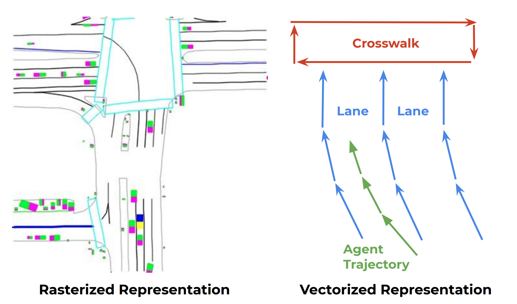
Fig 1. Illustration of the rasterized rendering (left) and vectorized approach (right) to represent high-definition map and agent trajectories. (Image source: https://arxiv.org/pdf/2005.04259.pdf)

Model Architecture

The authors attempt to encode various features of road networks via vectors. Road entities such as crosswalks, stop signs, lanes, and others, can be represented as points, polygons and curves. All these entities can further be represented as polylines. Finally, all these polylines can be represented as sets of vectors. For example, the trajectory of some agent could be represented as a set of vectors sampled along the path of motion.

In particular, each vector \(v_i\) belonging to a polyline \(P_j\) is a node in the graph with node features given by: \(v_i = [d_i^s, d_i^e, a_i, j]\) Where:

\(d_i^s\) and \(d_i^e\) are the coordinates of the starting and ending points of the vector
\(a_i\) corresponds to attribute features, such as object type (lane, stop sign, etc), timestamps for trajectories, or road features, such as speed limits.
\(j\) is the integer id of \(P_j\), the polyline to which the vector belongs.

Thus, a polyline is a set of vectors : \(P = \{v_1, v_2\cdots, v_P\}\)

There are two types of components of the network. One type which looks at interactions between nodes within a polyline, forming polyline subgraphs, and one which looks at the higher order interactions between the polylines themselves, denoted as the global graph.

Polyline Subgraphs

For a given polyline, \(P\), a single layer of subgraph propagation is formulated as : \(v*i^{(l+1)} = \varphi*{rel}(g*{enc}(v_i^{(l)}, \varphi*{agg}(\{g\_{enc}(v_j^{(l)})\}))\) Where:

\(v_i^{(l)}\) is the node feature for the \(l\)-th layer of the subgraph network
- Therefore, \(v_i^{(0)}\) denotes the input features, \(v_i\).
\(g_{enc}\) is a function that transforms the individual node features
- It is implemented as a MLP with the weights shared among all the nodes
- It has a single fully connected layer followed by layer normalization, followed by ReLU.
\(\varphi_{agg}\) aggregates the information from all the neighbouring nodes that surround the target node
- It is implemented as a maxpool operation
\(\varphi_{rel}\) is the relational operator among the node and its neighbours
- It is simply a concatenation operation

In summary, the overall function takes in all the neighbouring nodes to the target, encodes them as vectors, then performs a maxpool. It then encodes the current node and concatenates it with the result of the maxpooling operation.

Each layer of the network has different weights for \(g_{enc}\), but they are shared among the nodes.

Finally, to obtain the features for a polyline, the nodes along the polyline are maxpooled as : \(p = \varphi_{agg}(\{v_i^{(L_p)}\})\)

Global Graph

Given a set of polyline node features, \(\{p_1, p_2, \cdots, p_P\}\), the objective is to model the interaction between these polylines. This is given by :

\[\{p_i^{(l+1)}\} = \text{GNN}(\{p_i^{(l)}\}, A)\]

Where:

The polyline node features at a layer are given by \(\{p_i^{(l)}\}\)
\(\text{GNN}\) is a single layer of the graph neural network
- \(\text{GNN} (P) = \text{softmax} (P_QP_K^T)P_V\)
  Where \(P\) is the node feature matrix and \(P_Q, P_K, P_V\) are its linear projections.
\(A\) is the adjacency matrix for the set of polyline nodes.
- It can be assumed that the polyline graph is a fully connected graph and \(A\) can be computed using spatial distance as a heuristic.

Future trajectories can thus be decoded from the nodes corresponding to the moving agents \(v*i^{future} = \varphi*{traj}(p_i^{(L_t)})\) Where:

\(L_t\) is the total number of \(\text{GNN}\) layers.
\(\varphi_{traj}\) is the trajectory decoder implemented as an MLP.

Therefore the values produced by the last layer are passed through the decoder for each polyline that is being considered.

Auxiliary Task

An auxiliary objective is introduced to encourage the global interaction graph to better capture interactions among different trajectories and map polylines.

During training time, the model randomly masks out the features for a subset of polyline nodes, say, \(p_i\), and the objective is to recover the masked out features as : \(\hat{p*i} = \varphi*{node}(p_i^{(L_t)})\) Where:

\(\varphi_{node}\) is the node feature decoder implemented as an MLP. This is not used during inference.
\(p_i\) is a node from a fully connected unordered graph
To identify a polyline node when its features are masked out, the minimum values o the start coordinates of all the vectors that belong to it is computed. This becomes \(p_i^{id}\)
- The input node features are thus \(p_i^{(0)} = [p_i; p_i^{id}]\)

This task is similar to that used by the BERT language model that predicts missing tokens based on bidirectional data.

Overall Structure

The objective function is thus : \(L = L_{traj} + \alpha L_{node}\) Where:

\(L_{traj}\) is the negative Gaussian log-likelihood for the ground-truth future trajectories
\(L_{node}\) is the Huber loss between the predicted node features and the ground-truth masked node features
\(\alpha\) is a scalar that balances the two loss terms

Experiments

The authors tested the performance of VectorNet on one vehicle behaviour prediction benchmark, the Agroverse dataset.

Dataset

Argoverse motion forecasting is a dataset designed for vehicle behaviour prediction with trajectory histories. There are 333K 5-second long sequences split into 211K training, 41K validation and 80K testing sequences. The creators curated this dataset by mining interesting and diverse scenarios, such as yielding for a merging vehicle, crossing an intersection, etc. The trajectories are sampled at 10Hz, with (0, 2] seconds are used as observation and (2, 5] seconds for trajectory prediction. Each sequence has one “interesting” agent whose trajectory is the prediction target.

Metrics

The authors adopt the Average Displacement Error (ADE) computed over the entire trajectories and the Displacement Error at t (DE@ts) metric, where \(t\in \{1.0, 2.0, 3.0\}\) seconds. Additionally, the displacements are in meters.

Results

The performance of VectorNet on the Argoverse dataset is compared with several baseline approaches and a few state-of-the-art architectures, which is summarised in table 1.

Model	DE@3s	ADE
Constant Velocity	7.89	3.53
Nearest Neighbour	7.88	3.45
LSTM ED	4.95	2.15
Challenge Winter: uulm-mrm	4.19	1.90
Challenge Winter: Jean	4.17	1.86
VectorNet	\(\textbf{4.01}\)	\(\textbf{1.81}\)

Table 1. Trajectory prediction performance on the Argoverse Forecasting test set when number of sampled trajectories K=1. Results were retrieved from the Agroverse leaderboard on 03/18/2020

The baseline approaches are the constant velocity baseline, nearest neighbour retrieval and LSTM encoder-decoder. The state-of-the-art approaches are the winners of the Agroverse Forecasting Challenge. From table 1, VectorNet is able to outperform both state-of-the-art models in terms of DE@3s and ADE when K=1.

Visualization

Some of the predictions made by VectorNet on trajectories in the Agroverse dataset are visualized in Fig 2.

Artificial neural network

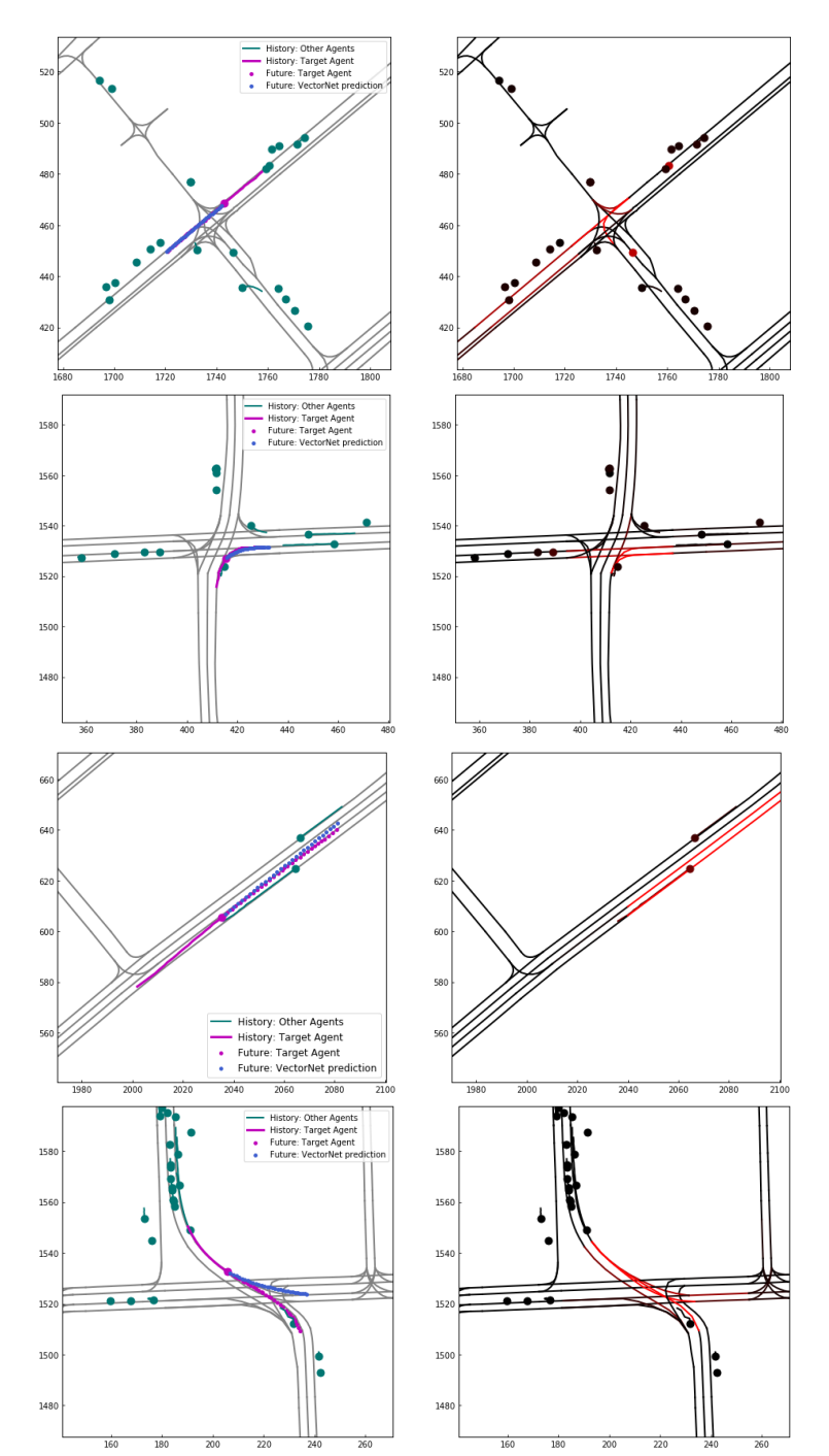
Fig 2. (Left) Visualization of the prediction: lanes are shown in grey, non-target agents are green, target agent’s ground truth trajectory is in pink, predicted trajectory in blue. (Right) Visualization of attention for road and agent: Brighter red colour corresponds to higher attention score. (Image source: https://arxiv.org/pdf/2005.04259.pdf)

It is observed that when argents are facing multiple choices (first two examples), the attention mechanism is able to focus on the correct choices (two right-turn lanes in the second example). The third example is a lane-changing agent, the attended lanes are the current lane and target lane. In the fourth example, though the prediction is not accurate, the attention still produces a reasonable score on the correct lane.

Takeaway

The main contribution of this paper is the method to encode HD maps and agent dynamics as vectors.

The paper proposes a novel hierarchical graph neural network with:

Level 1: aggregates information among vectors inside a polyline
Level 2: models the higher order relationships among polylines

The VectorNet is on-par in terms of performance with the best ResNet on the large scale in-house data set used by the researchers and is more computationally efficient.

It outperforms the best ConvNet on the publicly available Argoverse data set while having a lower computational cost.

Introduction

Artificial neural network

Fig 1. Illustration of the rasterized rendering (left) and vectorized approach (right) to represent high-definition map and agent trajectories. (Image source: https://arxiv.org/pdf/2005.04259.pdf)

Model Architecture

In particular, each vector \(v_i\) belonging to a polyline \(P_j\) is a node in the graph with node features given by: \(v_i = [d_i^s, d_i^e, a_i, j]\) Where:

\(d_i^s\) and \(d_i^e\) are the coordinates of the starting and ending points of the vector
\(a_i\) corresponds to attribute features, such as object type (lane, stop sign, etc), timestamps for trajectories, or road features, such as speed limits.
\(j\) is the integer id of \(P_j\), the polyline to which the vector belongs.

Thus, a polyline is a set of vectors : \(P = \{v_1, v_2\cdots, v_P\}\)

Polyline Subgraphs

For a given polyline, \(P\), a single layer of subgraph propagation is formulated as : \(v_i^{(l+1)} = \varphi_{rel}(g_{enc}(v_i^{(l)}, \varphi_{agg}(\{g_{enc}(v_j^{(l)})\}))\) Where:

\(v_i^{(l)}\) is the node feature for the \(l\)-th layer of the subgraph network
- Therefore, \(v_i^{(0)}\) denotes the input features, \(v_i\).
\(g_{enc}\) is a function that transforms the individual node features
- It is implemented as a MLP with the weights shared among all the nodes
- It has a single fully connected layer followed by layer normalization, followed by ReLU.
\(\varphi_{agg}\) aggregates the information from all the neighbouring nodes that surround the target node
- It is implemented as a maxpool operation
\(\varphi_{rel}\) is the relational operator among the node and its neighbours
- It is simply a concatenation operation

Each layer of the network has different weights for \(g_{enc}\), but they are shared among the nodes.

Finally, to obtain the features for a polyline, the nodes along the polyline are maxpooled as : \(p = \varphi_{agg}(\{v_i^{(L_p)}\})\)

Global Graph

Given a set of polyline node features, \(\{p_1, p_2, \cdots, p_P\}\), the objective is to model the interaction between these polylines. This is given by :

\[\{p_i^{(l+1)}\} = \text{GNN}(\{p_i^{(l)}\}, A)\]

Where:

The polyline node features at a layer are given by \(\{p_i^{(l)}\}\)
\(\text{GNN}\) is a single layer of the graph neural network
- \(\text{GNN} (P) = \text{softmax} (P_QP_K^T)P_V\)
  Where \(P\) is the node feature matrix and \(P_Q, P_K, P_V\) are its linear projections.
\(A\) is the adjacency matrix for the set of polyline nodes.
- It can be assumed that the polyline graph is a fully connected graph and \(A\) can be computed using spatial distance as a heuristic.

Future trajectories can thus be decoded from the nodes corresponding to the moving agents \(v_i^{future} = \varphi_{traj}(p_i^{(L_t)})\) Where:

\(L_t\) is the total number of \(\text{GNN}\) layers.
\(\varphi_{traj}\) is the trajectory decoder implemented as an MLP.

Therefore the values produced by the last layer are passed through the decoder for each polyline that is being considered.

Auxiliary Task

An auxiliary objective is introduced to encourage the global interaction graph to better capture interactions among different trajectories and map polylines.

During training time, the model randomly masks out the features for a subset of polyline nodes, say, \(p_i\), and the objective is to recover the masked out features as : \(\hat{p_i} = \varphi_{node}(p_i^{(L_t)})\) Where:

\(\varphi_{node}\) is the node feature decoder implemented as an MLP. This is not used during inference.
\(p_i\) is a node from a fully connected unordered graph
To identify a polyline node when its features are masked out, the minimum values o the start coordinates of all the vectors that belong to it is computed. This becomes \(p_i^{id}\)
- The input node features are thus \(p_i^{(0)} = [p_i; p_i^{id}]\)

This task is similar to that used by the BERT language model that predicts missing tokens based on bidirectional data.

Overall Structure

The objective function is thus : \(L = L_{traj} + \alpha L_{node}\) Where:

\(L_{traj}\) is the negative Gaussian log-likelihood for the ground-truth future trajectories
\(L_{node}\) is the Huber loss between the predicted node features and the ground-truth masked node features
\(\alpha\) is a scalar that balances the two loss terms

Experiments

The authors tested the performance of VectorNet on one vehicle behaviour prediction benchmark, the Agroverse dataset.

Dataset

Metrics

Results

The performance of VectorNet on the Argoverse dataset is compared with several baseline approaches and a few state-of-the-art architectures, which is summarised in table 1.

Model	DE@3s	ADE
Constant Velocity	7.89	3.53
Nearest Neighbour	7.88	3.45
LSTM ED	4.95	2.15
Challenge Winter: uulm-mrm	4.19	1.90
Challenge Winter: Jean	4.17	1.86
VectorNet	\(\textbf{4.01}\)	\(\textbf{1.81}\)

Table 1. Trajectory prediction performance on the Argoverse Forecasting test set when number of sampled trajectories K=1. Results were retrieved from the Agroverse leaderboard on 03/18/2020

Visualization

Some of the predictions made by VectorNet on trajectories in the Agroverse dataset are visualized in Fig 2.

Artificial neural network

Takeaway

The main contribution of this paper is the method to encode HD maps and agent dynamics as vectors.

The paper proposes a novel hierarchical graph neural network with:

Level 1: aggregates information among vectors inside a polyline
Level 2: models the higher order relationships among polylines

The VectorNet is on-par in terms of performance with the best ResNet on the large scale in-house data set used by the researchers and is more computationally efficient.

It outperforms the best ConvNet on the publicly available Argoverse data set while having a lower computational cost.

Colab Demo

https://colab.research.google.com/drive/1ldrHriSrpxNQ9t2igfBTdctp9pMUSYQw?usp=sharing

Introduction

One of the main things an autonomous vehicle needs to take into account is the pedestrians on the road. It needs to be able to learn general human movement and predict future trajectories.

In the past, human trajectories were modelled using hand-crafted functions for specific settings - such as to model attraction and repulsion. However, these approaches fail to generalize to more complex settings.

The authors of the paper propose a new architecture based on the LSTM model which can learn common rules and conventions of human movement without the need for any additional annotation of datasets.

Model Architecture

Problem Setup and Notation:

At time \(t\), the \(i^{th}\) person in the scene is represented by their XY-coordinates, \((x_t^i, y_t^i)\).
The positions of all the people are known from time \(1\) to \(T_{obs}\).
The objective is to predict their positions for times \(T_{obs+1}\) to \(T_{pred}\).

Model Architecture

The model uses one LSTM per person, with the weights shared across all sequences.

Pooling Strategy

To take into account the behaviour of all other sequences while predicting the trajectory of a given person, the authors implement a “Social” pooling strategy that connects the various LSTMs.

Suppose our objective is to predict the trajectory of the \(i^{th}\) agent. While predicting the trajectory at a given time step, we consider the neighbouring agents, and for each agent \(j\), the hidden state LSTM cell \(h_t^j\) of the agent is used to construct a hidden state tensor \(H_t^i\).

Formally, given a neighbourhood \(N_0\), and a hidden state dimension \(D\), construct a tensor for the \(i^{th}\) person :

\[H_t^{t} \in \mathbb{R}^{N_0 \times N_0 \times D}\]

given by :

\[H_t^i(m, n, :) = \sum_{j\in \mathcal{N}_i} 1_{mn}[x_t^j - x_t^i, y_t^j - y_t^i]h_{t-1}^j\]

Where:

\(h_{t-1}^j\) is the hidden state of the LSTM for the \(j^{th}\) person at time \(t-1\).
\(1_{mn}[x, y]\) is an indicator function to check if \((x, y)\) is in the cell \((m, n)\) of the grid.
\(\mathcal{N}_i\) is the set of neighbours corresponding to person \(i\).

So each grid cell corresponds to a certain distance from the agent \(i\). For each grid position, if a neighbouring trajectory is at that distance from \(i\), the hidden state for that trajectory at that time step is added to the tensor at that grid cell position. This is done for all neighbouring agents and for all grid cell positions.

Finally, the pooled social hidden states are embedded into \(a_i^t\) and the coordinates are embedded into \(e_i^t\). Formally :

\[e_t^i = \phi(x_t^i, y_t^i; W_e)\] \[a_i^t = \phi(H_t^i \; ; W_a)\] \[h_i^t = \text{LSTM}(h_i^{t-1}, e_i^t, a_t^i \; ; W_l)\]

Where :

\(\phi(.)\) is an embedding function with ReLU nonlinearity
\(W_e, W_a\) are the embedding weights
\(W_l\) are the weights of the LSTM.

Position Estimation

The hidden state at time \(t\) is used to predict the distribution of the trajectory position \((\hat{x}, \hat{y})^i_{t+1}\) at the next time step \(t+1\).

The authors assume that the coordinates are given by a bivariate Gaussian distribution parameterized by the bivariate mean, standard deviation, and correlation coefficient at time \(t+1\). Thus,

\[(\hat{x}, \hat{y})_t^i \sim \mathcal{N}(\mu_t^i, \sigma_t^i, \rho_t^i)\]

Where the Gaussian distribution parameters are predicted by a linear layer with a \(5\times D\) weight matrix \(W_p\) as follows :

\[[\mu_t^i, \sigma_t^i, \rho_t^i] = W_ph_i^{t-1}\]

The parameters of the LSTm are learned by minimizing the negative log-likelihood loss \(L_i\) for the \(i^{th}\) trajectory for each trajectory in the training data set.

Since the hidden states of all the LSTMs are coupled by the social pooling layer, backpropagation is jointly performed through multiple LSTMs in the scene at every time step.

Inference

During test time, the social LSTM model is used to predict the future position \((\hat{x}_t^i, \hat{y}_t^i)\) of the \(i^{th}\) person.

At each time step, the positions predicted by the social LSTM for each of the previous time steps is used as the input of the model instead of the true coordinates. These predicted coordinates also replace the true coordinates when constructing the social hidden state tensor.

Experiments

Datasets

The authors use two datasets which capture many real-world settings with thousands of non-linear trajectories. They also cover complex group dynamics such as couples walking together, groups crossing each other, and groups forming and dispersing.

ETH dataset : Contains two scenes with 750 different pedestrians
UCY dataset : Contains two scenes with 786 different people

Error Metrics:

The authors consider 3 error metrics :

Average displacement error : Mean Squared Error between the true and predicted trajectories.
Final Displacement error : Distance between the predicted and true final destinations at the end of the prediction period.
Average non-linear displacement error : MSE at the non-linear regions of a trajectory (since this is where most errors occur).

The authors observed that the social LSTM model outperformed the state-of-the-art methods on these publicly available datasets.

An example of a prediction made by the social LSTM is visualized in Fig 3. The scene consists of 4 individuals and the figure displays the predicted trajectories at a particular time.

Artificial neural network

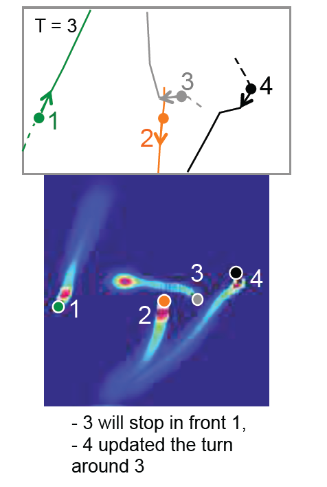
Fig 3. (Top) Input to the model : Solid lines are the ground truth trajectories, the dashed lines are the previous positions, and the dot is the current position. (Bottom) The output of the model as a probability of future positions. (Image source: https://openaccess.thecvf.com/content_cvpr_2016/html/Alahi_Social_LSTM_Human_CVPR_2016_paper.html)

Takeaways

The authors have proposed an LSTM based model that can jointly reason across multiple individuals to predict human trajectories in a scene. Each agent is assigned an LSTM and they share information through a novel social pooling layer.

The model outperforms other methods on public datasets and is capable of predicting several non-linear trajectories and group behaviours.

Introduction

Similar to Social LSTM, the authors of Social GAN seek to model pedestrian motions that are socially acceptable. While previous architectures such as the Social LSTM have made great progress, they suffer from two limitations. First and foremost, they fail to model interactions between all people in a scene efficiently. Instead, they model a local neighborhood around each person when making the prediction. Secondly, they tend to learn the “average behavior” since the loss function effectively minimizes the L2 norm between the ground truth and forecasted trajectories.

To address these shortcomings, the authors propose to use a Generative Adversarial Network (GAN) with a RNN Encoder-Decoder generator and a RNN based encoder discriminator. In addition, they propose a new pooling mechanism that learns a “global” pooling vector which encodes the subtle cues for all people involved in a scene.

Model Architecture

Problem Setup and Notation

The model receives as input all the trajectories for people in a scene as \(\textbf{X} = X_1, X_2, ..., X_n\) and predict the future trajectories \(\hat{\textbf{Y}} = \hat{Y}_1, \hat{Y}_2, ..., \hat{Y}_n\) of all people simultaneously.
The input trajectory of a person \(i\) is defined as \(X_i = (x_i^t, y_i^t)\) from time steps \(t=1, ..., t_{obs}\).
The future trajectory (ground truth) of a person \(i\) can similarly be defined as \(Y_i = (x_i^t, y_i^t)\) from time steps \(t = t_{obs} + 1, ..., t_{pred}\).

Generative Adversarial Networks

Generative Adversarial Networks (GANs) represent a paradigm shift in deep learning. Instead of training a single neural network to perform a certain task, GANs generally involve the training of two models in opposition to one another: a generator \(G\), whose primary objective is to capture the data distribution, as well as a discriminator \(D\), whose main goal is to estimate the probability that a sample came from the training data rather than \(G\). In more formal terms, the generator \(G\) takes a latent variable \(z\) as input and outputs sample \(G(z)\). The discriminator \(D\) takes a sample \(x\) and outputs \(D(x)\), the probability that the sample is real. The following objective function is used during training:

\[\min_G \max_D V(G, D) = E_{x\sim p_{data}(x)}[logD(x)] + E_{z\sim p(z)}[log(1-D(G(z)))]\]

Hence, the training procedure is akin to a two-player min-max game, in which the generator \(G\) is looking to minimize \(V(G, D)\) and the discriminator \(D\) is seeking to maximize \(V(G, D)\). A common application of GANs is in the area of Deepfake with the generator being responsible for generating deepfaked images and the discriminator responsible for determining whether the image is real or fake. Over the course of training, the generator will learn to generate more realistic images and the discriminator will get better at distinguishing between real and deepfaked images.

Socially-Aware GAN

The proposed model Socially-Aware GAN (SGAN) is effectively a GAN with a specialized pooling module. The SGAN model, therefore, consists of three main components: Generator (G), Pooling Module (PM) and Discriminator (D). A diagram of the SGAN model can be found in Fig 4.

Artificial neural network

Fig 4. Overview of the SGAN model. (Image source: https://arxiv.org/pdf/1803.10892.pdf)

\(\textbf{Generator.}\) The generator \(G\) of SGAN consists of an encoder and decoder. The encoder first uses a single layer MLP to obtain a fixed length vector \(e_i^t\), which is an embedding of the location of each person. These embeddings are then fed as input to the LSTM cell of the encoder at time \(t\), which is captured by the following recurrence relations:

\[e_i^t = \phi(x_i^t, y_i^t; W_{ee})\] \[h_{ei}^t = LSTM(h_{ei}^{t-1}, e_i^t; W_{encoder})\]

where \(\phi(\cdot)\) is the embedding function with ReLU nonlinearity, \(W_{ee}\) is the embedding weight. The LSTM weights (\(W_{encoder}\)) are shared between all people in a given scene.

The decoder is quite similar to the encoder in principle and can be described by the following recurrence relations:

\[e_i^t = \phi(x_i^{t-1}, y_i^{t-1}; W_{ed})\] \[P_i = PM(h_{d1}^{t-1}, ..., h_{dn}^t)\] \[h_{di}^t = LSTM(\gamma(P_i, h_{di}^{t-1}), e_i^t; W_{decoder})\] \[(\hat{x}_i^t, \hat{y}_i^t) = \gamma(h_{di}^t)\]

where \(\phi(\cdot)\) is the embedding function with ReLU nonlinearity, \(W_{ed}\) is the embedding weight. The LSTM weights are denoted by (\(W_{decoder}\)) and \(\gamma\) is an MLP. \(PM\) denotes the pooling module which will be discussed in a bit.

\(\textbf{Discriminator.}\) The discriminator \(D\) of SGAN consists of an encoder, which takes in \(T_{real} = [X_i, Y_i]\) or \(T_{fake} = [X_i, \hat{Y}_i]\) and classifies them as socially acceptable (real) or socially unacceptable (fake). A MLP is applied on the encoder’s last hidden state to obtain a classification score.

\(\textbf{Losses.}\) On top of the adversarial loss described previously, a L2 loss is applied on the predicted trajectory to measure how far are the generated samples from the actual ground truth. The total loss is the sum of the adversarial loss and the L2 loss.

Pooling Module

The pooling module proposed by the authors computes relative positions between the red and all other people as shown in Fig 5.

Artificial neural network

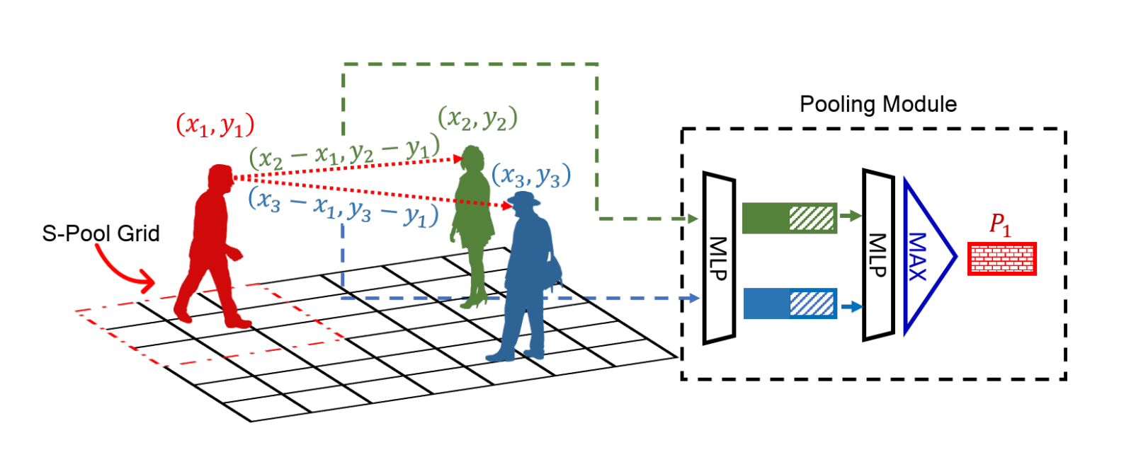
Fig 5. Comparison of the pooling module of SGAN (red dotted arrows) and Social Pooling of Social LSTM (red dashed grid). (Image source: https://arxiv.org/pdf/1803.10892.pdf)

These positions are concatenated with each person’s hidden state, processed independently by an MLP, then pooled elementwise using Max-Pooling to compute the red person’s pooling vector \(P_1\). The pooled vector \(P_i\) effectively summarizes all the information that a person needs to make a decision.

Encouraging Diverse Sample Generation

The authors propose a variety loss function that encourages the network to produce diverse samples. For each scene, \(k\) possible output predictions are generated by randomly sampling \(z\) from \(N(0, 1)\) and choosing the “best” prediction in L2 sense as the prediction. The variety loss can be described by the following equation:

\[L_{variety} = \min_k || Y_i - \hat{Y}_i^{(k)} ||_2\]

where \(k\) is a hyperparameter.

Experiments

Datasets

The authors evaluate the performance of SGAN on two publicly available datasets: ETH and UCY. These datasets consist of real world human trajectories with rich human-human interactions scenarios. There are 5 sets of data in total: ETH and HOTEL from the ETH dataset and UNIV, ZARA1, ZARA2 from the UCY dataset.

Evaluation Metrics

Similar to the authors of Social LSTM, the authors of SGAN evaluate their model on two error metrics:

Average Displacement Error (ADE): Average L2 distance between ground truth and the trajectory prediction over all predicted time steps
Final Displacement Error (FDE): The distance between the predicted final destination and the true final destination at the end of the prediction period \(T_{pred}\)

Both of these metrics are measured in meters.

Baselines

The authors of SGAN compare their model against the following baselines:

Linear: A linear regressor that estimates linear parameters by minimizing the least square error
LSTM: A simple LSTM with no pooling mechanism
S-LSTM: Social LSTM architecture proposed by Alahi et al, which is discussed in more detail in a previous section

Results

The results of SGAN are summarized in table 2. The author refer to their full method in this section as \(SGAN-kV-N\) where \(kV\) signifies if the model was trained under variety loss (\(k=1\) essentially means no variety loss) and \(N\) refers to the number of times the model is sampled during test time.

Metric	Dataset	Linear	LSTM	S-LSTM	\(\textbf{SGAN-1V-1}\)	\(\textbf{SGAN-20V-20}\)
	ETH	1.33	1.09	1.09	1.13	\(\textbf{0.81}\)
	HOTEL	\(\textbf{0.39}\)	0.86	0.79	1.01	0.81
ADE	UNIV	0.82	0.61	0.67	0.60	\(\textbf{0.60}\)
	ZARA1	0.62	0.41	0.47	0.42	\(\textbf{0.34}\)
	ZARA2	0.77	0.52	0.56	0.52	\(\textbf{0.42}\)
AVG		0.79	0.70	0.72	0.74	\(\textbf{0.58}\)
	ETH	2.94	2.41	2.35	2.21	\(\textbf{1.52}\)
	HOTEL	\(\textbf{0.72}\)	1.91	1.76	2.18	1.61
FDE	UNIV	1.59	1.31	1.40	1.28	\(\textbf{1.26}\)
	ZARA1	1.21	0.88	1.00	0.91	\(\textbf{0.69}\)
	ZARA2	1.48	1.11	1.17	1.11	\(\textbf{0.84}\)
AVG		1.59	1.11	1.52	1.54	\(\textbf{1.18}\)

Table 2. Quantitative results of all methods across datasets. The results reported are performed on trajectories with \(t_{pred}=12\)

From table 2, \(SGAN-1V-1\) performs worse than LSTM and S-LSTM in every metric as each predicted sample can be any of the multiple possible future trajectories. Moreover, the authors come to the conclusion that samples generated by \(SGAN-1V-1\) did not capture all possible scenarios.

On the contrary, \(SGAN-20V-20\) outperforms all other models in every metric as the variety loss encourages the network to produce diverse samples. The fact that the predicted samples are sampled multiple times also help account for all the plausible future predictions. However, the authors did point out that simply drawing more samples without the variety loss does not result in a significant improvement in performance.

Takeaways

The main contribution from this paper is that GANs are well suited to modeling socially acceptable trajectories along with the proposal of two novel ideas:

A Pooling Module that is capable of learning a “global” pooling vector which encodes information about all people in a scene
Variety loss that encourages the generation of more diverse predictions

The results illustrate that SGAN is able to outperform all other architectures in human trajectory prediction, and the Pooling Module encourages the model to predict more “socially” plausible paths.

Video Demo

https://colab.research.google.com/drive/1ldrHriSrpxNQ9t2igfBTdctp9pMUSYQw?usp=sharing

Reference

Please make sure to cite properly in your work, for example:

[1] Gao, Jiyang, et al. “Vectornet: Encoding hd maps and agent dynamics from vectorized representation.” Proceedings of the IEEE/CVF Conference on Computer Vision and Pattern Recognition. 2020.

[2] Alahi, Alexandre, et al. “Social lstm: Human trajectory prediction in crowded spaces.” Proceedings of the IEEE conference on computer vision and pattern recognition. 2016.

[3] Gupta, Agrim, et al. “Social gan: Socially acceptable trajectories with generative adversarial networks.” Proceedings of the IEEE Conference on Computer Vision and Pattern Recognition. 2018.

Code Repository

[1] Reimplement VectorNet

[2] Social LSTM Implementation in PyTorch

[3] Social GAN

Introduction

Paper 1: VectorNet - Encoding HD Maps and Agent Dynamics From Vectorized Representation

Introduction

Model Architecture

Polyline Subgraphs

Global Graph

Auxiliary Task

Overall Structure

Experiments

Dataset

Metrics

Results

Visualization

Takeaway

Introduction

Model Architecture

Polyline Subgraphs

Global Graph

Auxiliary Task

Overall Structure

Experiments

Dataset

Metrics

Results

Visualization

Takeaway

Colab Demo

Paper 2: Social LSTM: Human Trajectory Prediction in Crowded Spaces

Introduction

Model Architecture

Problem Setup and Notation:

Model Architecture

Pooling Strategy

Position Estimation

Inference

Experiments

Datasets

Error Metrics:

Takeaways

Paper 3: Social GAN: Socially Acceptable Trajectories with Generative Adversarial Networks

Introduction

Model Architecture

Problem Setup and Notation

Generative Adversarial Networks

Socially-Aware GAN

Pooling Module

Encouraging Diverse Sample Generation

Experiments

Datasets

Evaluation Metrics

Baselines

Results

Takeaways

Video Demo

Reference

Code Repository