Text Guided Art Generation

Our project mainly works on investigating and innovating a text-guided image generation model and an art painting model and connecting the two models together to create artworks with only text inputs. Some artists have already applied AI/Deep Learning in their art creation (VQGAN-CLIP), while the development of diffusion models and transformers may provide more stable and human-like output. In this project, we will talk about how we utilized VQGAN + CLIP and Paint Transformer for the whole generating pipeline and present Colab demos.

• Introduction
• Technical Details of Models
  • AutoEncoder
  • VQVAE
  • Transformer
  • VQGAN
  • VQGAN + CLIP
  • Paint Transformer
• Implementation
  • VQGAN + CLIP
  • Paint Transformer
  • Combine Two Models
• Demo
• Spolight Presentation
• Code Repository and Innovation
• Reference

Introduction

Our project idea is inspired by Paint Transformer which turns a static image into an oil painting drawing process and VQGAN + CLIP Art generation which turns texts into artwork. We want to combine the idea from both projects and design a model which could give an artistic painting process from the text described. Specifically, we want to reproduce and explain VQGAN+CLIP for text-guided image generation and take it as the input of the Paint Transformer to produce an artwork with paint strokes.

To clarify, VQGAN + CLIP is actually the combination of two models: VQGAN stands for Vector Quantized Generative Adversarial Network, which is a type of GAN that can be used to generate high-resolution images; while CLIP stands for Contrastive Language-Image Pretraining, which is a classifier that could pick the most relevant sentence for the image from several options. Unlike other attention GAN, which can also generate images from text, VQGAN + CLIP is more like a student-teacher pair: VQGAN will generate an image, and CLIP will judge whether this image has any relevance to the prompt and tell VQGAN how to optimize. In this blog, we will focus more on the generative portion and take CLIP as a tool for the text-guided art generation process.

Paint Transformer is a neural network model which mimicking real human oil painting process given a traget image.

Technical Details of Models

AutoEncoder

Autoencoder is a type of neuron network frequently used to learn the representations of images. Similar to what we have in the Fast R-CNN model in object detection, it has an encoder that maps the input image to a representation tensor normally named as latent vector, shown as the yellow box in Fig 1, and a decoder that upsamples the latent vector, or more intuitively, revert the encoding to reconstruct the original image. If we can find an encoder-decoder combination that can minimize the reconstruction loss, then we can compress the image into the latent vector for other operations without significant loss so that we can use resources more efficiently. In Fast R-CNN, we do ROI proposals over the code instead of the original image. This is an unsupervised learning technique, meaning that we don’t use the labels of images to compute the loss.

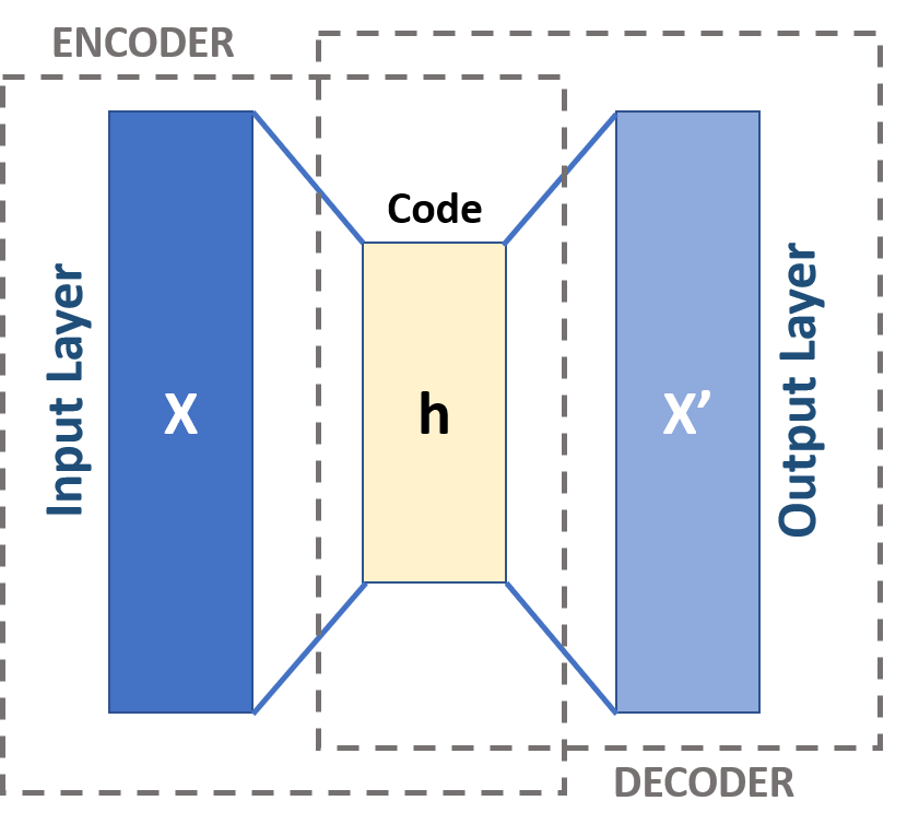
Fig 1. High level architecture of an autoencoder [5].

For tje encoder, the structure would be the same as any normal neuron network we used for image classification without the last few fully-connected layers (otherwise we will lose too much information), including MLP (only linear layers), CNN, and ResNet. For the decoder, we can use a combination of max unpooling, linear layers with increasing inputs, or transposed convolutional layer if the encoder is constructed with CNN or ResNet for upsampling. A simple example of an autoencoder in Pytorch is shown below:

class AutoEncoderConv(torch.nn.Module):
  def __init__(self):
    super().__init__()

    # Encoder
    self.encoder_conv1 = torch.nn.Sequential(
        torch.nn.Conv2d(3, 16, 3, 1, 1),
        torch.nn.ReLU(),
        torch.nn.Conv2d(16, 16, 3, 1, 1),
        torch.nn.ReLU()
    )

    self.encoder_conv2 = torch.nn.Sequential(
        torch.nn.Conv2d(16, 32, 3, 1, 1),
        torch.nn.ReLU(),
        torch.nn.Conv2d(32, 32, 3, 1, 1),
        torch.nn.ReLU()
    )

    self.encoder_conv3 = torch.nn.Sequential(
        torch.nn.Conv2d(32, 64, 3, 1, 1),
        torch.nn.ReLU(),
        torch.nn.Conv2d(64, 64, 3, 1, 1),
        torch.nn.ReLU()
    )

    # Decoder
    self.decoder_conv1 = torch.nn.Sequential(
        torch.nn.ConvTranspose2d(64, 64, 3, 1, 1),
        torch.nn.ReLU(),
        torch.nn.ConvTranspose2d(64, 32, 2, 2, 0),
        torch.nn.ReLU()
    )

    self.decoder_conv2 = torch.nn.Sequential(
        torch.nn.ConvTranspose2d(32, 32, 3, 1, 1),
        torch.nn.ReLU(),
        torch.nn.ConvTranspose2d(32, 16, 2, 2, 0),
        torch.nn.ReLU()
    )

    self.decoder_conv3 = torch.nn.Sequential(
        torch.nn.ConvTranspose2d(16, 16, 3, 1, 1),
        torch.nn.ReLU(),
        torch.nn.ConvTranspose2d(16, 3, 2, 2, 0),
        torch.nn.Sigmoid()
    )

  def forward(self, x):
    x = self.encoder_conv1(x)
    x = F.max_pool2d(x, 2)
    x = self.encoder_conv2(x)
    x = F.max_pool2d(x, 2)
    x = self.encoder_conv3(x)
    code = F.max_pool2d(x, 2)
    x = self.decoder_conv1(code)
    x = self.decoder_conv2(x)
    x = self.decoder_conv3(x)
    return x

We can optimize the model based on the return value x. Training this model over CIFAR-10, we can get an 0.56 average training loss in 15 epochs. However, there is the main drawback: since it is optimizing the mapping between the input image and the latent vector, it works well for training images but worse for others. To have a broader usage setting, we need the variational autoencoder(VAE).

VQVAE

Differ from the standard autoencoder, variational autoencoder tries to find a probability distribution of the latent vector instead of a mapping. VAEs also have encoders and decoders like autoencoders, but since the latent space is now a continuous distribution, we also need to optimize the parameters of this distribution. The idea was firstly introduced by Diederik P. Kingma and Max Welling [7] under the context of Bayesian estimation: assume the input data \(\mathbf{x}\) has an unknown distribution \(P(x)\). We know guess that it is a normal distribution with parameter group \(\theta\) (it can be a mean and a variance, or multiple of them to get a mixture of normal distribution). We start from \(\mathbf{z}\) as an initial guess of the parameters (usually called the latent encoding). Let \(p_{\theta}(\mathbf{x}, \mathbf{z})\) be the joint probability. The marginal probability of \(\mathbf{x}\) is

Where \(p_\theta (\mathbf{x} \vert \mathbf{z})\) is the probability decoder and \(p_\theta (\mathbf{z})\) is the prior of latent space. However, integrating all \(\mathbf{z}\) is intractable. Alternatively, by the Bayes’ rule,

In every iteration, we can compute this posterior and use it as the prior for the next iteration. Since we don’t know the real \(\theta\), we just use our own estimate codebook \(\Theta\) and optimize it gradually.

The original VAE uses normal distribution as the proposal of the underlying phenomenon, but in Vector-Quantized VAE (VQVAE), the parameters are several tensors (embedding) with fixed length called Codebook and use a data compression method “vector quantization” to generate the latent encoding. What this method basically does is to find the embedding vector with the lowest distance to the flattened tensors before quantization, store the corresponding index, and replace them with those embedding vectors. Mathematically, the quantized latent vector has the formula

where \(Z\) is the codebook, \(z_{ij}\) is a flatten tensor after encoder, and \(z_q\) is the quantized latent vector [3].

Concerning the calculation of loss, there are three types of losses: reconstruction loss, which basically calculates the distance between the reconstructed image and original image; stop-gradient loss for embedding, which optimize the embedding network; and commitment loss, which optimizes the encoder. The last two loss is specifically for the vector quantization. The overall loss is the sum of three, which is

where \(G\) is the decoder(generator), \(\hat{x}\) is the reconstructed image, and \(sg[\cdot]\) stands for stop gradient.

Transformer

So far we have the model to learn local interactions between image pixels. The original paper for VQGAN [3] also mentioned that long-range interactions are also important for high-resolution image synthesis and image recovery. We would like to know what pixel would be next given all pixels we perceived previously. This idea is similar to the next-word prediction in NLP using transformer models. A revolutionary idea in VQGAN architecture is using a partial GPT-2 transformer model to train the long-range interaction.

Transformer is a model mainly based on the self-attention mechanism in NLP, which the model would put more weight (attention) on certain portions, similar to how humans perceive and understand a sentence. Fig 2 is a diagram of the architecture of a transformer.

Fig 2. The transformer architecture (VQGAN only uses the decoder part since vector quantization has already produce the encoding) [8].

For VQGAN, only the decoder will be used, since vector quantization in VQVAE has already generated both latent vector and the encoding at the same time. The encoding is a long discrete sequence of numbers, and the goal of transformer is to predict each number in the sequence based on all previous numbers with the maximum likelihood. Specifically, we want to find

Where \(s_i\) is the ith number in the sequence [9]. Therefore, the loss function of this transformer would be \(\mathbb{E}(-\log{(\Pi_{i} p(s_i\vert s_{<i}))})\), which is the negative-log loss.

VQGAN

Combining all models above together, we can finally build the VQGAN with the following architecture:

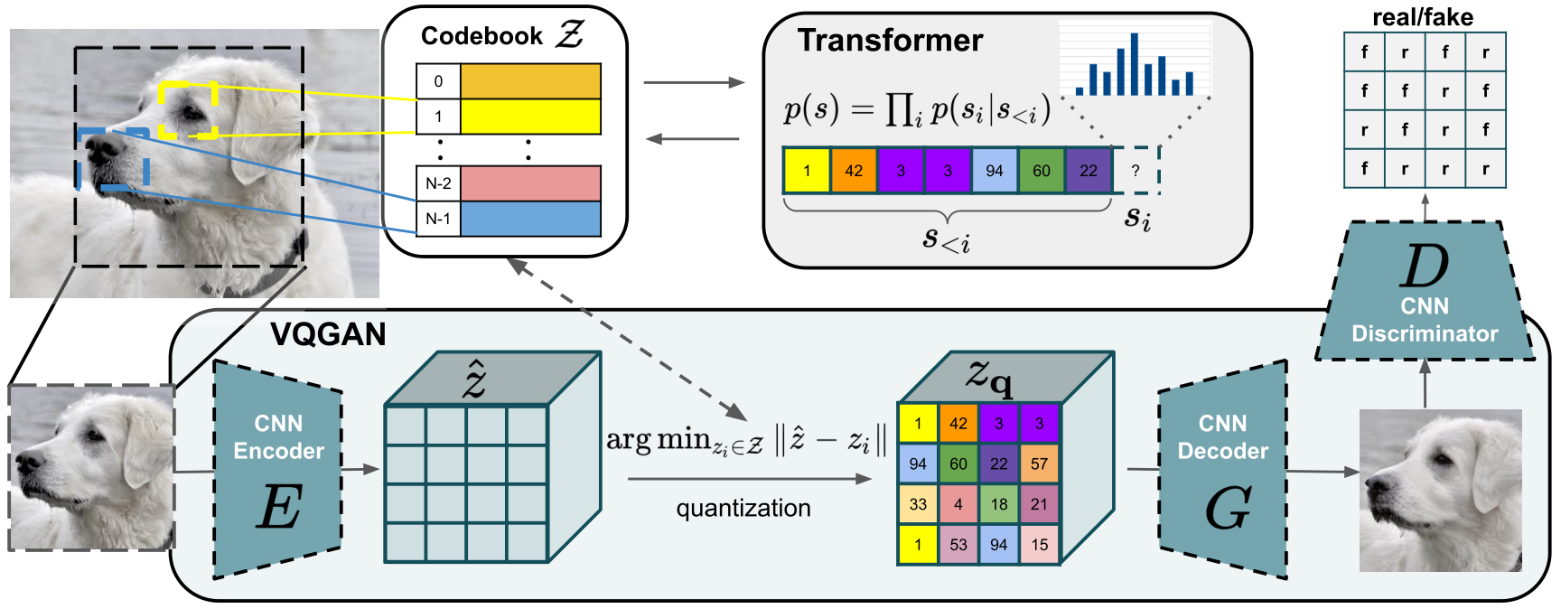
Fig 3. Overall VQGAN Architecture [8].

We still miss a component: the discriminator. In GAN, during training, there is usually one generator to construct the target image, and a discriminator, which is nothing but a classifier, that is used to distinguish whether the image is real or fake and compute the loss. Both generator and discriminator optimize and compete with each others so that we can get better performance on the generator. In VQGAN, a convolutional discriminator will take the image generated by VQVAE (the generator) and output a real-fake matrix, which is a square matrix with 0’s and 1’s. For the project, since we are training on CIFAR-10, where each image only has \(32\times 32\) dimension, it still works well even we only output a single true-false bit from the discriminator.

For the loss function, we use the minmax loss, which is commonly used for GAN:

where \(D\) is the discriminator, and \(\hat{x}\) is the reconstructed image. When training the whole VQGAN without the transformer, we need to add the loss from VQVAE and this loss with some adaptive coefficient. In our implementation, we have 7 epoch warm up stages which the adversarial loss will not contribute in the optimization, then apply the loss with a coefficient 0.001, since the discriminator may not perform well at the beginning, and introduce loss too early may cause overconfidence of the generator.

Lastly, for the training procedure, we first train the VQVAE with a discriminator to obtain the best latent codebook that can represent the distribution of the image. After that, we train the transformer based on the codebook and encoder to model the long-range interaction. When generating the image, the original method is having a sliding window of fixed size over a region and only predicting pixels with the neighbors in the window. This would allow parallelism and save more resources, but since we would only generate a \(32\times 32\) as the demo, it is reasonable to directly predict over the whole image.

VQGAN + CLIP

To incorporate VQGAN with CLIP to provide the power of image generation from text, we will download the pretrained CLIP model from OpenAI (reimplement it would time consuming and may not obtain the same performance). For VQGAN, we only need the decoder and the codebook. Our goal is trying to find a latent vector before vector quantization that can produce a figure corresponding to the text prompt. Initially, we randomly generate a latent vector with min and max bounded by the minimum and maximum in the codebook. Then the pretrained CLIP model will parse the prompt into tokens and encode them. It also outputs the weight of token and constructs a Prompt object for loss calculation. Each Prompt object behaves like a self-attention unit that computes the distance between CLIP prediction on the generated image and the embedding and scales by a weight.

During training, the system will first quantize the latent vector, decode it to a normalized image, perform an augmentation, and output encoding by the CLIP model. We then put the output into each Prompts to calculate the loss. Finally, based on the loss, we optimize the latent vector and repeat the operation. Fig 4 shows the complete workflow:

Fig 4. Workflow of VQGAN+CLIP text-guided image generation.

Paint Transformer

Paint transformer is a novel Computer Vision Algorithm that converts a static picture into an artistic oil painting. It can also generates the whole painting process from an empty canvas. The Demo section shows our modification of this algorithm according to the original paper.

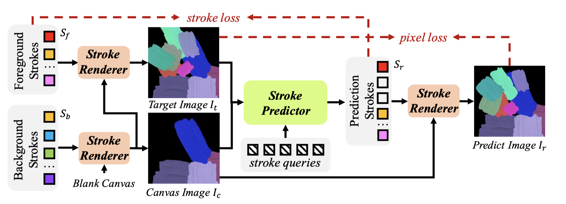
Fig 5. Framework of Paint Transformer [2].

Paint Transformer Framework

The structure of the whole painting pipeline is provided in Fig 5. The Paint Transformer contains two parts: Stroke Predictor and Stroke Renderer. For each rendering iteration, the Stroke Predictor will give predictions from the input image I_t, and pass the result to the stroke renderer. The stroke render will add strokes accordingly from the Canvas images I_c. The result will be the image I_r.

Loss function

Both stroke (direction, dimension, and sequence) and pixel (color) will affect the result. The loss function contains the two factors are presented below:

The pixel loss is just the \(L_1\) distance between pixels:

The stroke loss involces more parameters. For two strokes \(s_u\) and \(s_v\)

• L1 stroke distances \(\mathcal{D}^{u,v}_{L_1}\)
• Wasserstein stroke distances (for rotational strokes) \(\mathcal{D}^{u,v}_W\)
• Binary cross entropy loss (for indicating confidence of the predicted stoke) \(\mathcal{D}^{u,v}_{bce}\)
• Weight terms \(\lambda_{L_1}\), \(\lambda_{W}\), \(\lambda_{bce}\)

The loss function for stokes is:

where X and Y are the optimal permutations for predicted strokes and target strokes (ground truth) given by the Hungarian algorithm.

According to this loss function, actually any pictures can be used for input and training. So Paint Transformer does not require any dataset during the training process. For foreground and background strokes can be generated by random sampling.

Stroke Render

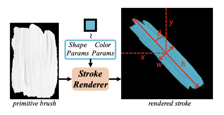
Fig 6. Stroke transformation [2].

Fig 6 showed the mechanism of a Stroke Render which takes a predefined brush prototype and transforms it into expected stroke by applying different coordinates (x,y), height(h), width(w), rotate angle(\(\theta\)), and color (r,g,b). The renderer only contains linear transformation, so it is not trainable.

Stroke Predictor

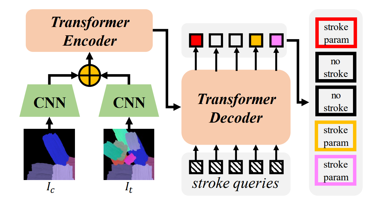
Fig 7. Stroke predictor framework [2].

Fig 7 illustrates the framework of the Stroke Predictor. The goal of the Stroke Predictor is to predict a set of strokes to draw images from the canvas image I_c to the target image I_t. Convolutional neural network on I_c and I_t gives out feature maps and positional information of two images, which are used for comparing differences and generating predicted strokes in the encoder. In the below code snippet, the self.enc_img represents the CNN for target image (I_t) and the self.enc_canvas represents the convolutional neural network for the canvas (I_c). The convolutional network encoder implementation is implemented as followed:

class Painter(nn.Module):

    def __init__(self, param_per_stroke, total_strokes, hidden_dim, n_heads=8, n_enc_layers=3, n_dec_layers=3):
        super().__init__()
        self.enc_img = nn.Sequential(
            nn.ReflectionPad2d(1),
            nn.Conv2d(3, 32, 3, 1),
            nn.BatchNorm2d(32),
            nn.ReLU(True),
            nn.ReflectionPad2d(1),
            nn.Conv2d(32, 64, 3, 2),
            nn.BatchNorm2d(64),
            nn.ReLU(True),
            nn.ReflectionPad2d(1),
            nn.Conv2d(64, 128, 3, 2),
            nn.BatchNorm2d(128),
            nn.ReLU(True))
        self.enc_canvas = nn.Sequential(
            nn.ReflectionPad2d(1),
            nn.Conv2d(3, 32, 3, 1),
            nn.BatchNorm2d(32),
            nn.ReLU(True),
            nn.ReflectionPad2d(1),
            nn.Conv2d(32, 64, 3, 2),
            nn.BatchNorm2d(64),
            nn.ReLU(True),
            nn.ReflectionPad2d(1),
            nn.Conv2d(64, 128, 3, 2),
            nn.BatchNorm2d(128),
            nn.ReLU(True))
        self.conv = nn.Conv2d(128 * 2, hidden_dim, 1)
        self.transformer = nn.Transformer(hidden_dim, n_heads, n_enc_layers, n_dec_layers)
        self.linear_param = nn.Sequential(
            nn.Linear(hidden_dim, hidden_dim),
            nn.ReLU(True),
            nn.Linear(hidden_dim, hidden_dim),
            nn.ReLU(True),
            nn.Linear(hidden_dim, param_per_stroke))
        self.linear_decider = nn.Linear(hidden_dim, 1)
        self.query_pos = nn.Parameter(torch.rand(total_strokes, hidden_dim))
        self.row_embed = nn.Parameter(torch.rand(8, hidden_dim // 2))
        self.col_embed = nn.Parameter(torch.rand(8, hidden_dim // 2))
    def forward(self, img, canvas):
        b, _, H, W = img.shape
        img_feat = self.enc_img(img)
        canvas_feat = self.enc_canvas(canvas)
        # More transformation code continues, you could check out our code base

Only Stroke Predictor contains trainable parameters. So the training part will only focus on optimizing the encoder part of the Stroke Predictor.

Dataset Selection

In the paper, authors used a novel way to train the model with existing datasets. According to framework of this project, the loss function is the comparison between the generated strokes and the original image. Without dependencies on labels, randomly generated images can be used for training. Since there is no limit of generating random images, the dataset can be really large for training more reliable models. The following snippet shows the generation of a random image. The foreground and alpha serve as a random stroke and pixel generator and assign corresponding value to old (which later becomes I_c and I_t through further transformation)

old = torch.zeros(self.opt.batch_size // 4, 3, self.patch_size * 2, self.patch_size * 2, device=self.device)
for i in range(self.opt.used_strokes):
    foreground = foregrounds[:, i, :, :, :]
    alpha = alphas[:, i, :, :, :]
    old = foreground * alpha + old * (1 - alpha)
old = old.view(self.opt.batch_size // 4, 3, 2, self.patch_size, 2, self.patch_size).contiguous()
old = old.permute(0, 2, 4, 1, 3, 5).contiguous()
self.old = old.view(self.opt.batch_size, 3, self.patch_size, self.patch_size).contiguous()

Painting Process

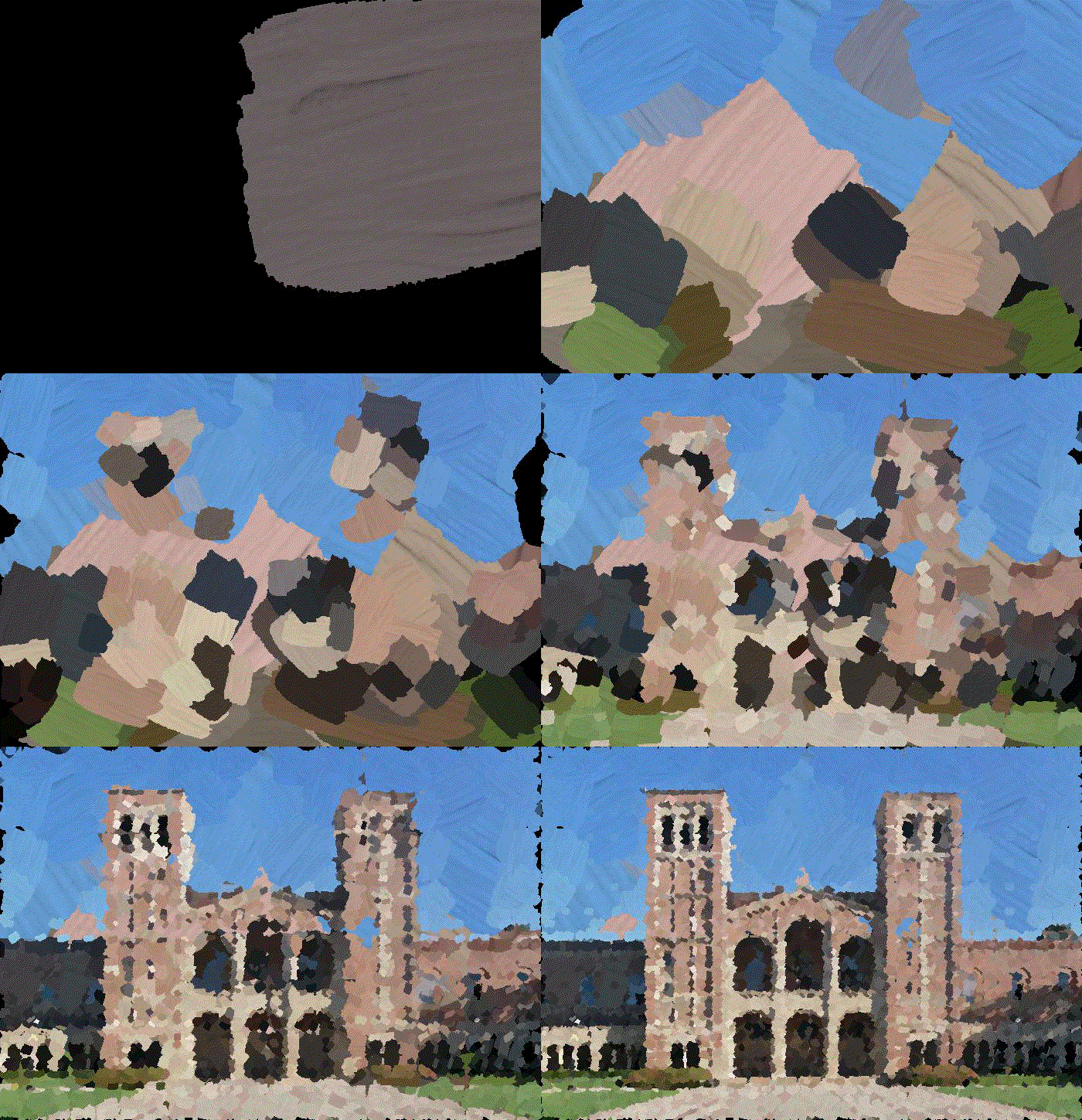
After training, the whole pipeline can be used for mimicking a real-world painting process. The Demo section illustrates the painting process. The drawer will run K iterations to finish the drawing. The value of K depends on the input picture dimension and can be derived through the below formula:

\(K = \text{max}(\text{argmin}_K\{P \times 2^K \geq \text{max}(H,W)\},0)\) The below algorithm shows the drawing algorithm given an input image.

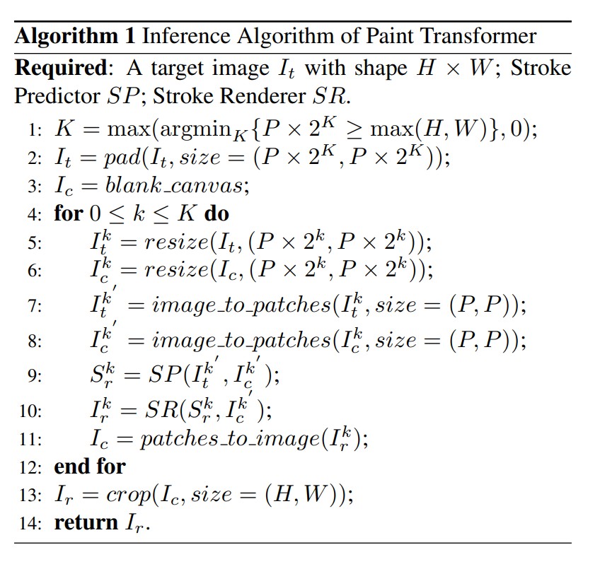
Fig 8. Drawing process algorithm [2].

According to Fig 8, starting from the empty canvas, some strokes will be added to the canvas each iteration. Each iteration of painting is based on the last iteration’s result and new strokes will be added through Stroke Predictor and Stroke Render.

Implementation

VQGAN + CLIP

All models for this system are trained using CIFAR-10, where each image has shape \(32 \times 32 \times 3\). The encoder is a combination of ConvNet and ResNet without batch normalization (experiment found that normalization and changing activation function perform worse since it will cause loss of information). It has 128 hidden channels in the ConvNet and 2 Resnet block layers. Inversely, the decoder is a combination of transposed convolution layer and ResNet, with 128 hidden channels and 2 residual block layers. Before entering the vector quantization module, an additional ConvNet will downsample the features. The vector quantization module has 512 embedding vectors, each has 64 elements. The discriminator is a normal CNN with batch normalization and fully-connected layers. Each ConvNet layer is activated by a Leaky Relu function. During training, we apply a 6 epoch warm up to ignore adversarial loss and obtain an improvement of performance by decreasing loss from 0.15 to 0.12.

When training the transformer, we encode the prediction output from the transformer into one hot matrix and calculate the cross-entropy loss of each step. Since we only have 64 elements in the input sequence, the transformer will predict the next element based on the previous 1~63 elements. Fig 8 shows the performance, where the first image is the generated output, the second one is the original decoded image, and the third one is the cropped input image. There is some degree of prediction, even though it is not that well.

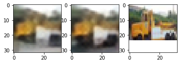
Fig 9. Image recovery based on 1/8 cropped image.

Vector quantization:

# permute dimension: BCHW -> BHWC
z = z.permute(0,2,3,1).contiguous()
z_shape = z.shape

#flatten
flat_z = z.reshape(-1, self.emb_dim)
l2_dist = (torch.sum(flat_z**2, dim=1, keepdim=True) 
        + torch.sum(self.emb.weight**2, dim=1) 
        - 2 * torch.matmul(flat_z, self.emb.weight.t()))

# find closest embedded vector with index and generate 1-hot matrix
enc_idx = torch.argmin(l2_dist, dim=1).unsqueeze(1)
enc = torch.zeros(enc_idx.shape[0], self.num_emb, device=z.device)
enc.scatter_(1, enc_idx, 1)

z_q = torch.matmul(enc, self.emb.weight).reshape(z_shape)

For the connection with CLIP, most of the generating codes and utilities are borrowed from the original Google Colab file. The performance is not that good due to training on the low-resolution image, but it still correctly generate features of objects, including colors and shapes. It works better for items in the category of CIFAR-10.

Prompt: banana

Prompt: red car

Prompt: airplane

Paint Transformer

Dataset Selection:

The original approach in the code was the no dataset approach. We reimplemented and modified the training code to enable the external dataset approach for comparison. Below are choices of datasets we used for training:

• Original no-dataset approach (20000 random samples)
• Miniplaces (10000 samples in the test set)
• Landscape Pictures (4319 samples)

Training

For each dataset, we trained a Paint Transformer Model for about 3 hours on an RTX 3080 graphics card. Due to different dataset sizes, we could achieve 120 to 220 epochs of training.

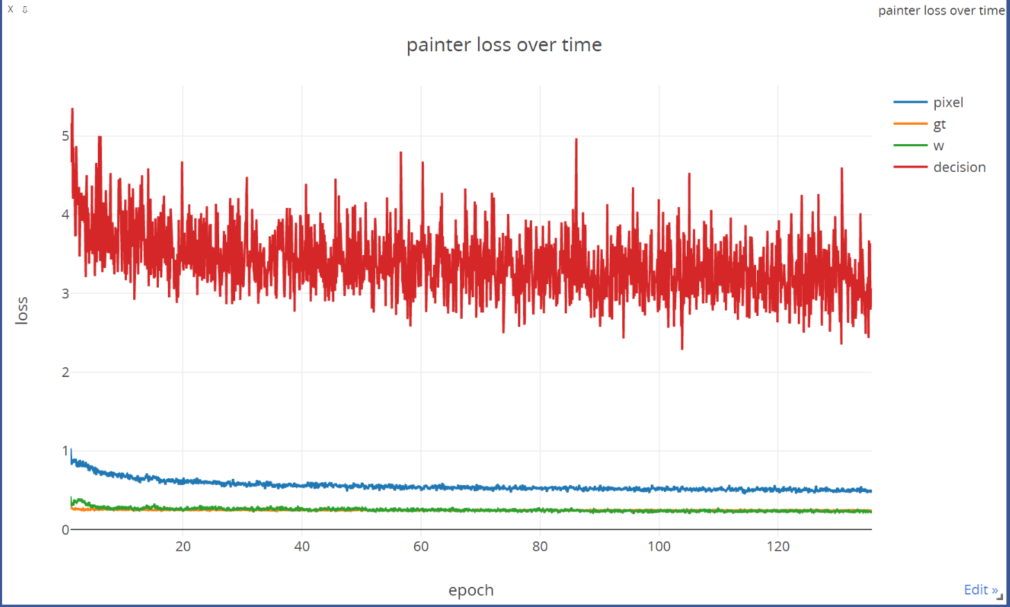Fig 10. Loss curve when we are using Miniplaces dataset for training.

The loss trend is shown in Fig 10 shows the loss curve during the training process for Miniplaces dataset. Other datasets (including the random dataset) have a similar trend. According to the loss curve, the convergence happens around 80-100 epochs.

Result:

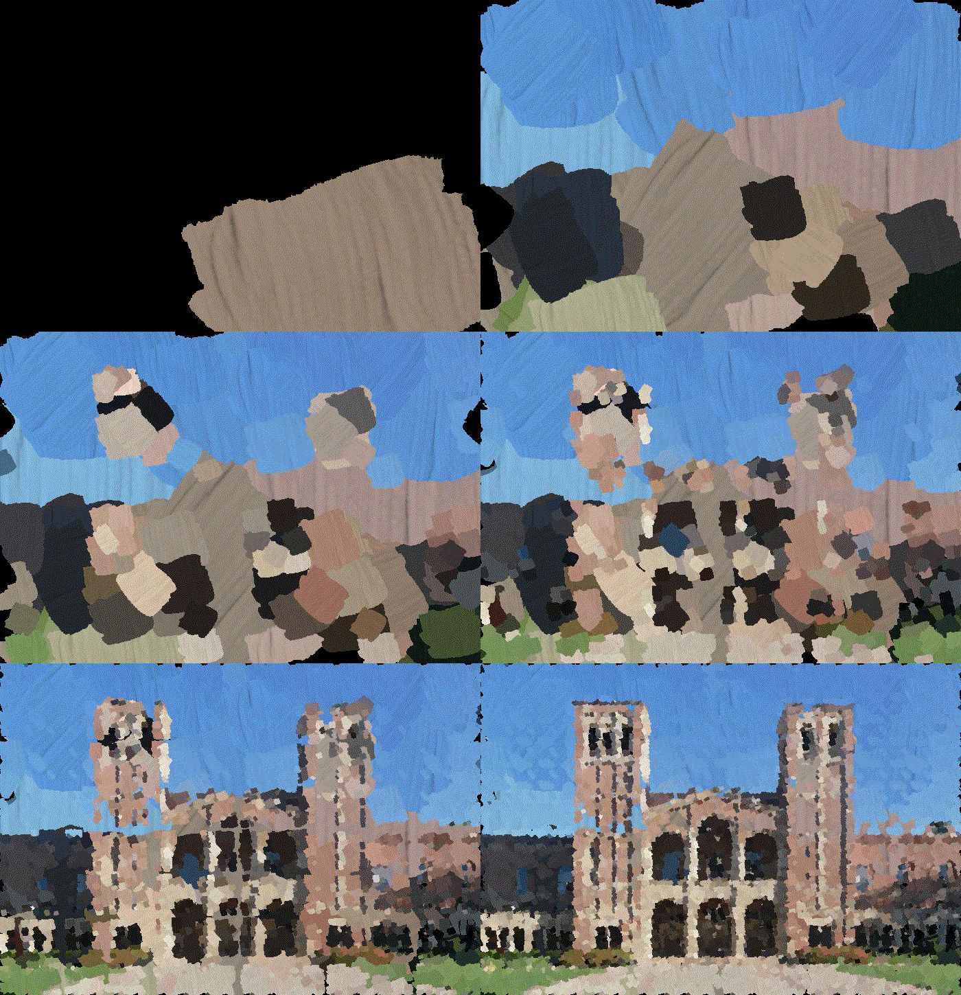
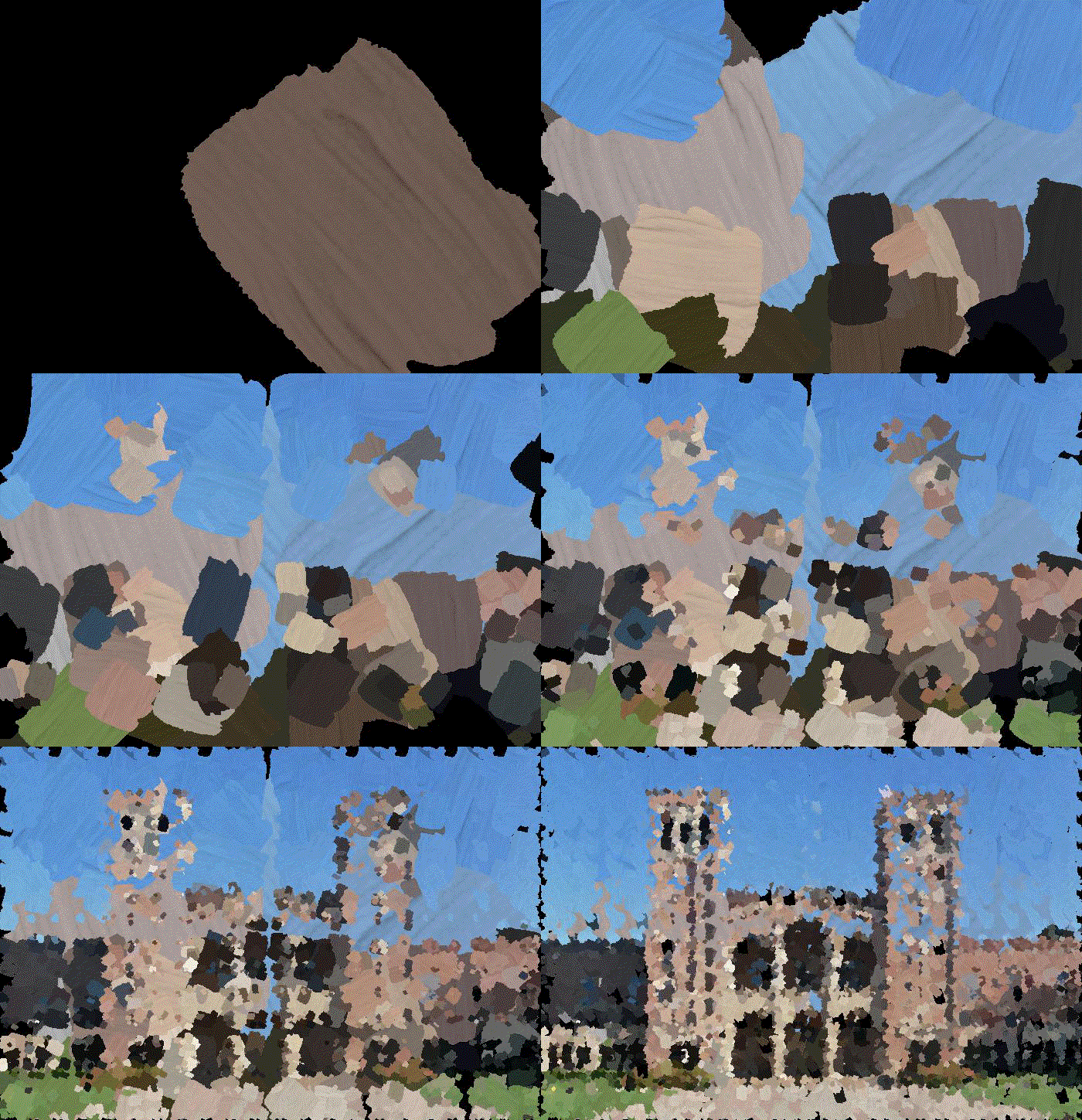
Below are oil paintings generated from the original pretained model given in the code repository and three different models trained by us using 120 epochs.

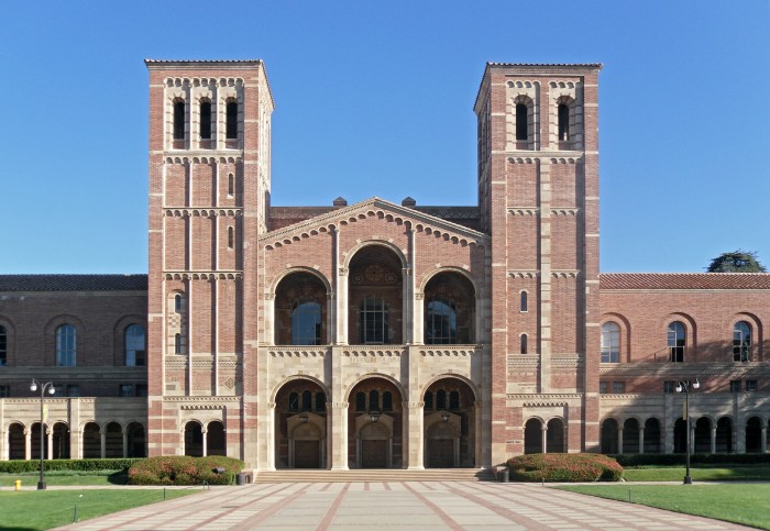Fig 11. Original input image (UCLA Royce Hall).

Input	Output	Drawing Process
Pretained model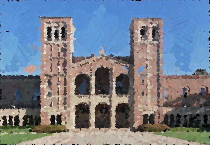
No-dataset approach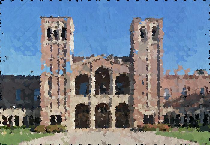
Miniplaces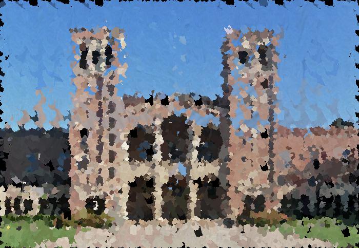
Landscape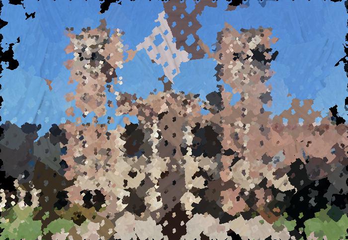

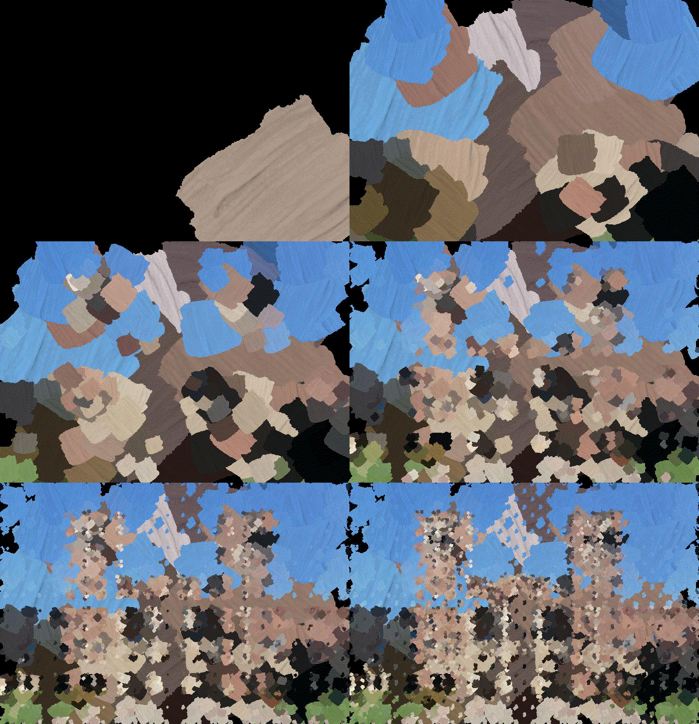Table 1. Paintings outputted from each model.

Summary:

Among all three results, the result from the no-dataset approach actually performed the best. Our implementation and modification of the no dataset model performed better than the Miniplaces dataset model in terms of painting quality. We could conclude that the number of samples outweighed the quality of the dataset in creating a better model, which aligns with the statement in the paper that the no-dataset approach can achieve equivalent performance without extra training time.

Combine Two Models

For better visual appearance, we will use the pretrained model in taming-transformer, with a more detailed prompt to guide the image generation. The result is shown in the video below:

Prompt: a painting of a rabbit on the grass

After producing the generated image, we further pass the image into the Paint Transformer to generate the picture with paining strokes. The final output given text prompt is displayed in Fig 12.

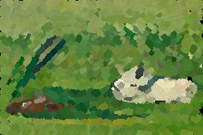
Fig 12. Output of Paint Transformer for the picture generated by VQGAN+CLIP.

Demo

Code base: Google Drive

VQGAN + CLIP demo: Colab

Paint Transformer demo: Colab

Spolight Presentation

Slides: Google Docs

Code Repository and Innovation

[1] VQGAN + CLIP Art generation

[2] AttnGAN

[3] PaintTransformer

For VQGAN + CLIP, we innovated our original training code (use CIFAR-10 dataset) and demo code in Colab. The demo has both pretrained model and our own model option. For Paint Transformer, we modified the training code to accept outside dataset and wrote demo code in Colab. We did an ayalysis of benefits of their no dataset approach comparing to our original models in this blog.

Reference

[1] Xu, Tao, et al. “Attngan: Fine-grained text to image generation with attentional generative adversarial networks.” Proceedings of the IEEE conference on computer vision and pattern recognition. 2018.

[2] Liu, Songhua, et al. “Paint transformer: Feed forward neural painting with stroke prediction.” Proceedings of the IEEE/CVF International Conference on Computer Vision. 2021.

[3] Esser, Patrick, Robin Rombach, and Bjorn Ommer. “Taming transformers for high-resolution image synthesis.” Proceedings of the IEEE/CVF Conference on Computer Vision and Pattern Recognition. 2021.

[4] Kim, Gwanghyun, and Jong Chul Ye. “Diffusionclip: Text-guided image manipulation using diffusion models.” arXiv preprint arXiv:2110.02711 (2021).

[5] Michela Massi - Own work, CC BY-SA 4.0, https://commons.wikimedia.org/w/index.php?curid=80177333

[6] Rath, Sovit Ranjan.”Getting Started with Variational Autoencoder using PyTorch.” https://debuggercafe.com/getting-started-with-variational-autoencoder-using-pytorch/

[7] Kingma, Diederik P., and Max Welling. “Auto-encoding variational bayes.” arXiv preprint arXiv:1312.6114 (2013).

[8] Dive Into Deep Learning. “10.7. Transformer.” https://d2l.ai/chapter_attention-mechanisms/transformer.html

[9] Miranda Lj. “The Illustrated VQGAN.” https://ljvmiranda921.github.io/notebook/2021/08/08/clip-vqgan/#perception

[10] Van Den Oord, Aaron, and Oriol Vinyals. “Neural discrete representation learning.” Advances in neural information processing systems 30 (2017).