Enhanced Self-Driving with Vision Based model.
Self-driving is a hot topic for deep vision applications. However, Vision-based urban driving is hard. Lots of methods for learning to drive have been proposed in the past several years. In this work, we focus on reproducing “Learning to drive from a world on rails” and trying to solve the drawbacks of the methods such as high pedestrian friction rate. We will also utilize the lidar(which is preinstalled on most cars with some self-driving capability) data to achieve better benchmark results.
Demo
Video Demo
Colab Demo
Introduction
Our work is a continuation of Learning to drive from a world on rails which uses dynamic programming to learn an agent from past driving logs and then applies it to generate action values. This work is also very closely related to Learning by Cheating which uses a similar two-stage approach to tackle the learning problem. At the same time, we will compare our work with a few others that use a totally different approach such as ChauffeurNet: Learning to Drive by Imitating the Best and Synthesizing the Worst that learns to drive by synthesizing images to deal with the worst case scenario. In our work, we will try to solve the drawbacks of “Learning to drive from a world on rails” which doesn’t use the most accurate Lidar data and has a high pedestrian friction rate problem.
Technical Details
Overview
In order to acquire a autonomous drive agent, we divide the work into the following 3 steps:
- Train a Kinematic forward model
- Based on predefined reward values, compute Q values using Bellman Updates
- With the supervision of precomputed Q values, generate the final model based policy
In terms of training data and evaluation, they are all sampled from the CARLA traffic simulator.
Simulator
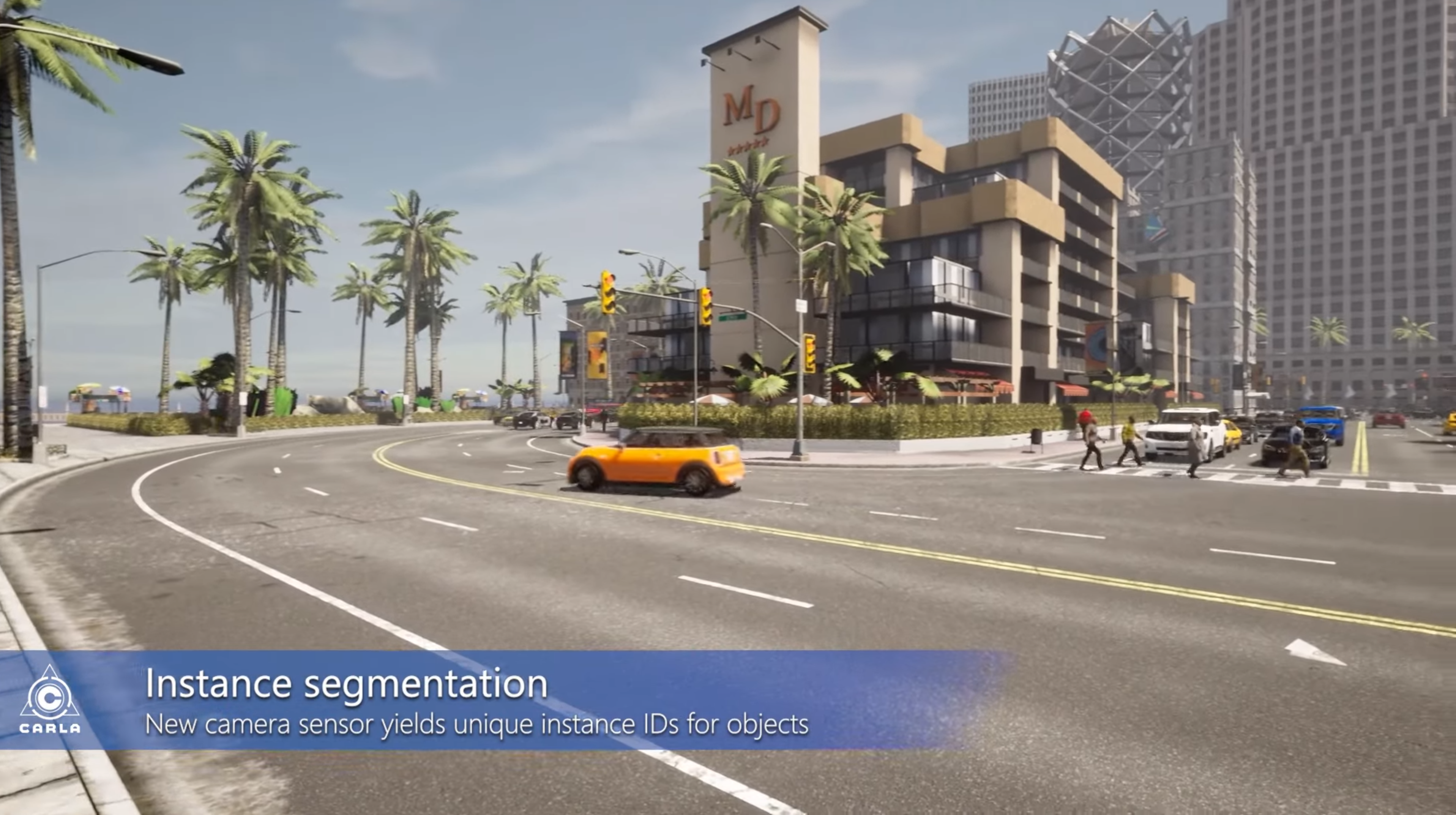
In our work, we use the same traffic simulator(CARLA) as many other similar papers. CARLA has been developed from the ground up to support development, training, and validation of autonomous driving systems. In addition to open-source code and protocols, CARLA provides open digital assets (urban layouts, buildings, vehicles) that were created for this purpose and can be used freely. The simulation platform supports flexible specification of sensor suites, environmental conditions, full control of all static and dynamic actors, map generation, and much more.
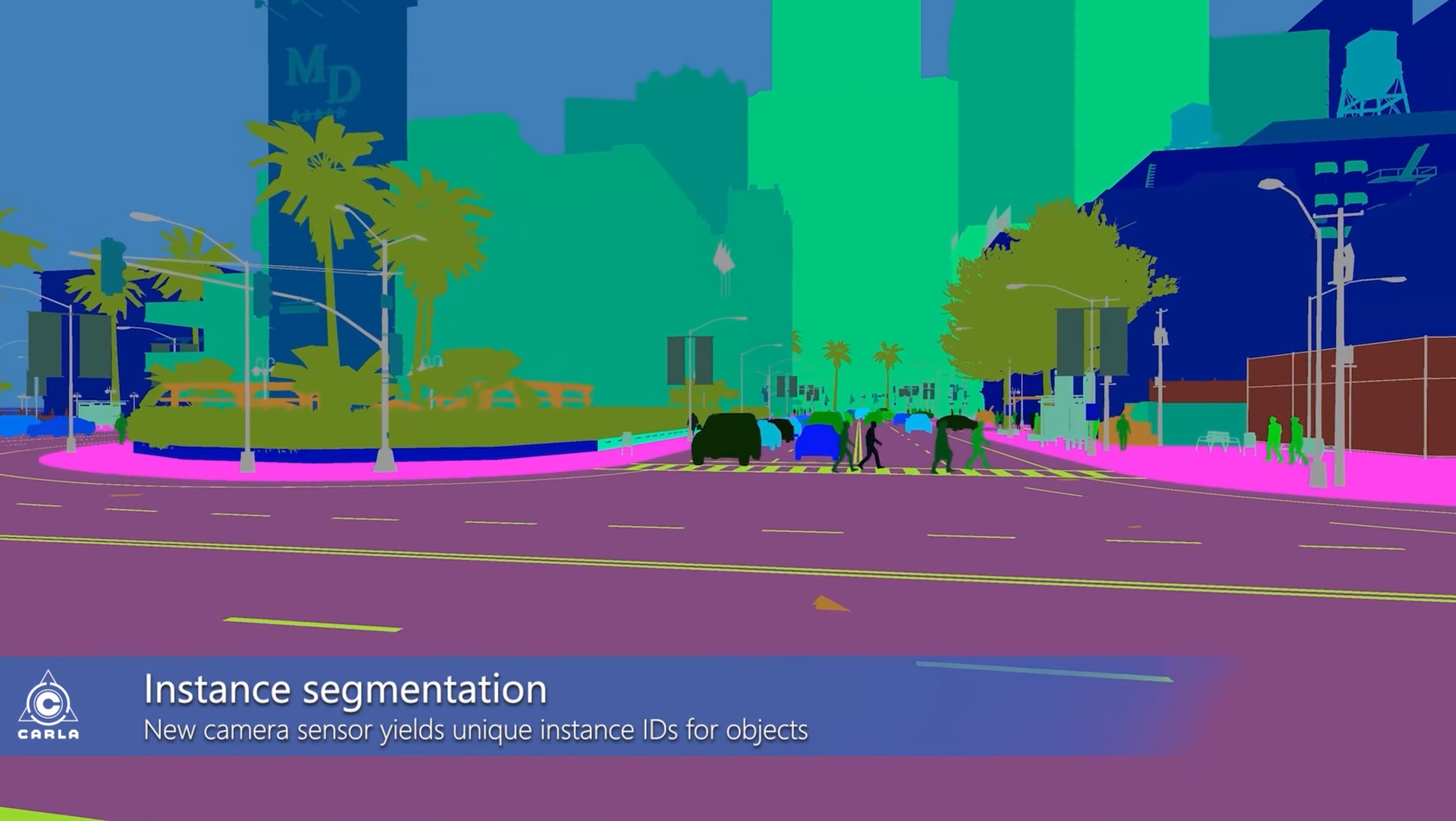
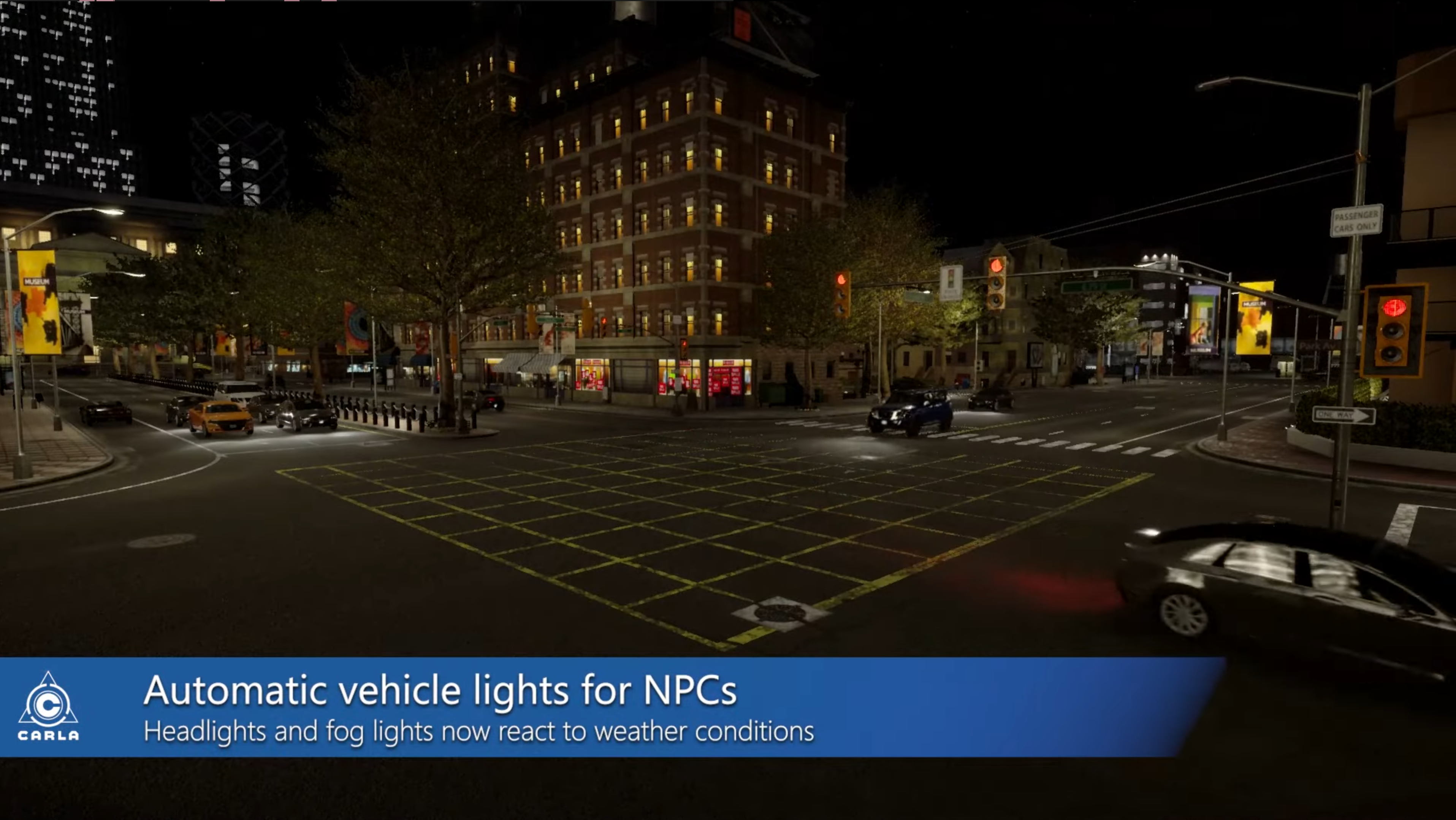
Below are a few advantages that CARLA brings to us.
| CARLA Simulator | Instance Segmentation | Different Lighting |
|---|---|---|
 |
 |
 |
Forward Kinematic Model
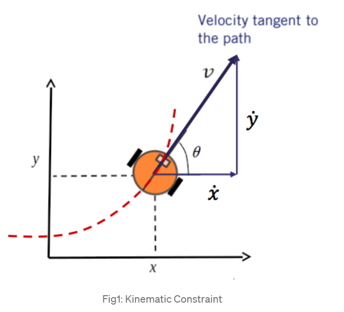
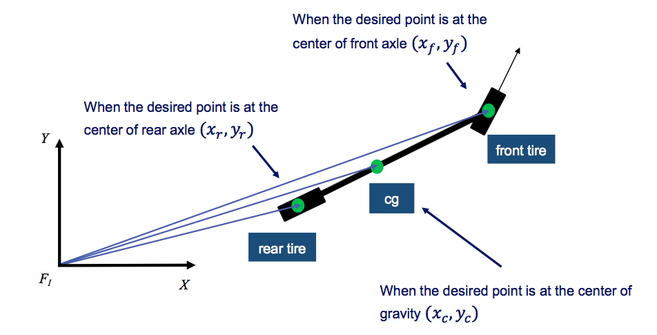
The goal of the forward model is to take as inputs the current ego-vehicle state as 2D location, orientation and speed and predict the next ego-vehicle state, orientation, and speed. In this work, a parameterized bicycle model is used as the structural prior. The basic parameters in a bicycle model are shown on the right.
The bicycle model is called the front wheel steering model, as the front wheel orientation can be controlled relative to the heading of the vehicle. Our target is to compute state [x, y, 𝜃, 𝛿], 𝜃 is heading angle, 𝛿 is steering angle. Our inputs are [𝑣, 𝜑], 𝑣 is velocity, 𝜑 is steering rate.
To analyze the kinematics of the bicycle model, we must select a reference point X, Y on the vehicle which can be placed at the center of the rear axle, the center of the front axle, or at the center of gravity or cg.
Below is the implementation of Kinematic bicycle model in PyTorch
class EgoModel(nn.Module):
    def __init__(self, dt=1./4):
        super().__init__()

        self.dt = dt

        # Kinematic bicycle model
        self.front_wb = nn.Parameter(torch.tensor(1.),requires_grad=True)
        self.rear_wb  = nn.Parameter(torch.tensor(1.),requires_grad=True)

        self.steer_gain  = nn.Parameter(torch.tensor(1.), requires_grad=True)
        self.brake_accel = nn.Parameter(torch.zeros(1), requires_grad=True)
        self.throt_accel = nn.Sequential(
            nn.Linear(1,1,bias=False),
        )

    def forward(self, locs, yaws, spds, acts):

        '''
        only plannar
        '''

        steer = acts[...,0:1]
        throt = acts[...,1:2]
        brake = acts[...,2:3].byte()

        accel = torch.where(brake, self.brake_accel.expand(*brake.size()), self.throt_accel(throt))
        wheel = self.steer_gain * steer

        beta = torch.atan(self.rear_wb/(self.front_wb+self.rear_wb) * torch.tan(wheel))

        next_locs = locs + spds * torch.cat([torch.cos(yaws+beta), torch.sin(yaws+beta)],-1) * self.dt
        next_yaws = yaws + spds / self.rear_wb * torch.sin(beta) * self.dt
        next_spds = spds + accel * self.dt

        return next_locs, next_yaws, F.relu(next_spds)
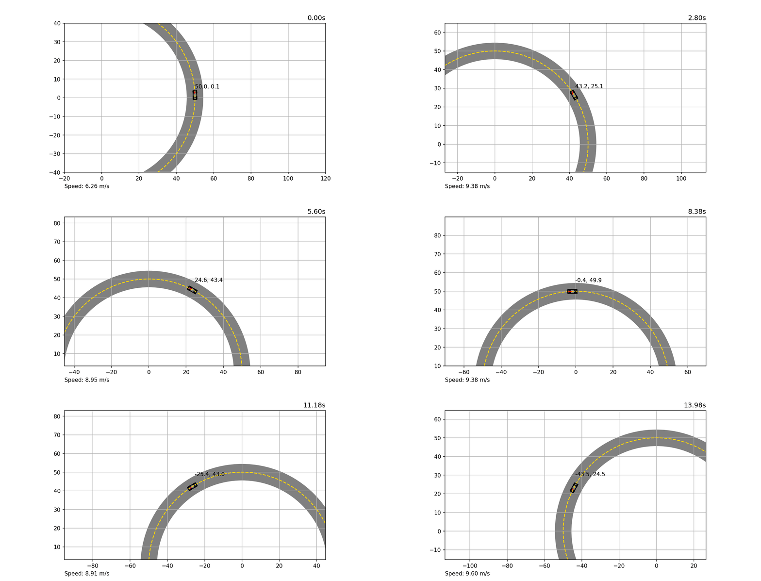
Here is a demo of the trained Kinematic model
Bellman Equation Evaluation
As the vehicle state in autonomous driving is continuous, it’s impossible to model each state. Therefore, a discretization method is used to represent the reward of each state. For each time-step t, the value function is represented as a 4D tensor which is discretized into \(N_H * N_W\) position bins,\(N_v\) velocity bins and \(N_{\theta}\) orientation bins. The value function and action value function can be described by the following 2 equations
\[V(L_{t}^{ego}, \hat{L}_t^{world}) = \underset{a}{max}Q(L_t^{ego}, \hat{L}_t^{world}, a)\] \[Q(L_t^{ego}, \hat{L}_t^{world}, a_t) = r(L_t^{ego}, \hat{L}_t^{world}, a_t) + \gamma V(T^{ego}(L_t^{ego}, \hat{L}_t^{world}, a), \hat{L}_{t+1}^{world})\]The action-value function is needed for all ego-vehicle state \(L^{ego}\), but only recorded world states \(\hat{L}_t^{world}\). Therefore, it’s sufficient to evaluate the action-value function on just recorded world states for all ego-vehicle: \(\hat{V}_t(L_t^{ego}) = V(L_t^{ego}, \hat{L}_t^{world}), \hat{Q}_t(L_t^{ego}, a_t) = V(L_t^{ego}, \hat{L}_t^{world}, a_t).\) Furthermore, since the world states are strictly ordered in time, hence the Bellman equation simplifies to
\[V(L_{t}^{ego}) = \underset{a}{max}Q(L_t^{ego}, a)\] \[Q(L_t^{ego}, a_t) = r(L_t^{ego}, \hat{L}_t^{world}, a_t) + \gamma V(T^{ego}(L_t^{ego}, a))\]It’s easy to observe that the above equation uses the compact states(position, orientation, and velocity) of the vehicle. Therefore, it can be solved using backward induction and dynamic programming.
Below is the main implementation of computing Q values
@staticmethod
def compute_table(ref_yaw, device=torch.device('cuda')):

    ref_yaw = torch.tensor(ref_yaw).float().to(device)

    next_locs = []
    next_yaws = []
    next_spds = []

    locs = torch.zeros((ref_yaw.shape)+(2,)).float().to(device)

    action = BellmanUpdater._actions.expand(len(BellmanUpdater._speeds),len(BellmanUpdater._orient),-1,-1).permute(2,0,1,3)
    speed  = BellmanUpdater._speeds.expand(len(BellmanUpdater._actions),len(BellmanUpdater._orient),-1).permute(0,2,1)[...,None]
    orient = BellmanUpdater._orient.expand(len(BellmanUpdater._actions),len(BellmanUpdater._speeds),-1)[...,None]

    delta_locs, next_yaws, next_spds = BellmanUpdater._ego_model(locs, orient+ref_yaw, speed, action)

    # Normalize to grid's units
    # Note: speed is orientation-agnostic
    delta_locs = delta_locs*PIXELS_PER_METER
    delta_yaws = torch.atan2(torch.sin(next_yaws-ref_yaw-BellmanUpdater._orient[0]), torch.cos(next_yaws-ref_yaw-BellmanUpdater._orient[0]))
    delta_yaws = delta_yaws[...,0,0]/(BellmanUpdater._max_orient-BellmanUpdater._min_orient)*BellmanUpdater._num_orient

    next_spds = (next_spds[...,0,0]-BellmanUpdater._min_speeds)/(BellmanUpdater._max_speeds-BellmanUpdater._min_speeds)*BellmanUpdater._num_speeds

    return delta_locs, delta_yaws, next_spds
Model Based Policy
Based on the Q values computed in the above section, we are able to train a model based policy that generates the final vehicle operating commands. The process to generate the policy can be divided into the following 2 parts.
Visual Based Action Prediction
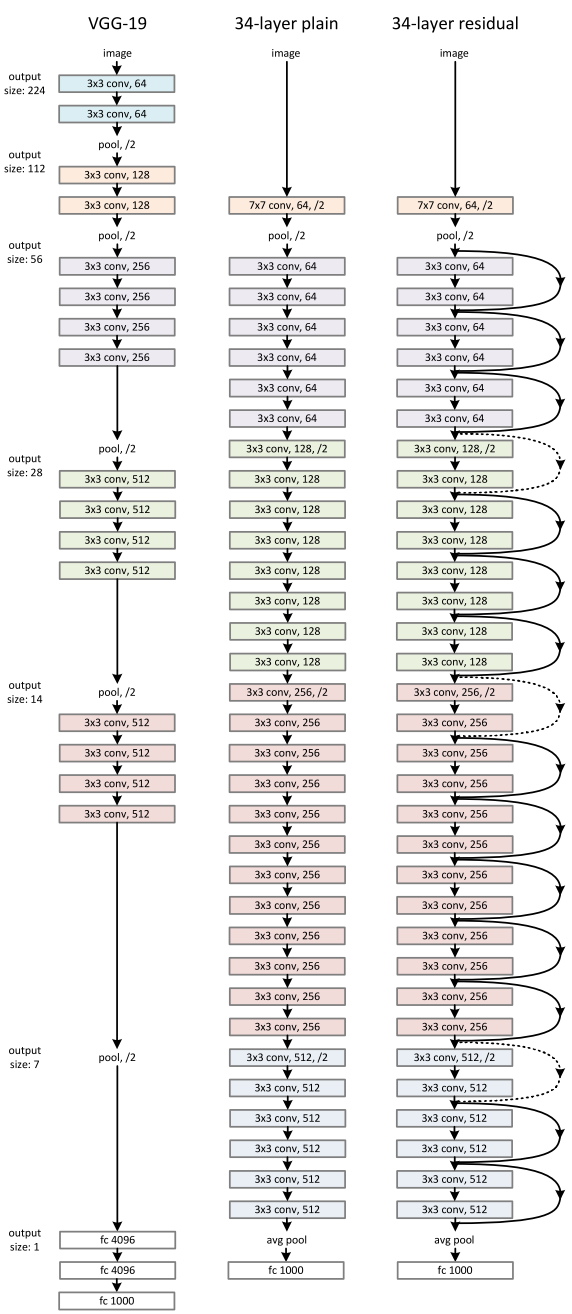
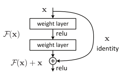
The policy network uses a ResNet34 backbone to parse the RGB inputs. And a global average pooling is used to flatten the ResNet Features before concatenating them with the ego-vehicle speed and feeding it into a fully connected network.
| ResNet34 | ResBlock |
|---|---|
 |
 |
The network produces a categorical distribution over the discretized action space. In CARLA, the agent receives a high-level navigation command \(c_t\) for each time step. We supervise the visuomotor agent simultaneously on all the high-level commands.
The code to build a ResNet34 can be implemented as below
class ResNet34(nn.Module):
    def __init__(self):
        super(ResNet34,self).__init__()

        self.block1 = nn.Sequential(
            nn.Conv2d(1,64,kernel_size=2,stride=2,padding=3,bias=False),
            nn.BatchNorm2d(64),
            nn.ReLU(True)
        )

        self.block2 = nn.Sequential(
            nn.MaxPool2d(1,1),
            ResidualBlock(64,64),
            ResidualBlock(64,64,2)
        )

        self.block3 = nn.Sequential(
            ResidualBlock(64,128),
            ResidualBlock(128,128,2)
        )

        self.block4 = nn.Sequential(
            ResidualBlock(128,256),
            ResidualBlock(256,256,2)
        )
        self.block5 = nn.Sequential(
            ResidualBlock(256,512),
            ResidualBlock(512,512,2)
        )

        self.avgpool = nn.AvgPool2d(2)
        # vowel_diacritic
        self.fc1 = nn.Linear(512,11)
        # grapheme_root
        self.fc2 = nn.Linear(512,168)
        # consonant_diacritic
        self.fc3 = nn.Linear(512,7)

    def forward(self,x):
        x = self.block1(x)
        x = self.block2(x)
        x = self.block3(x)
        x = self.block4(x)
        x = self.block5(x)
        x = self.avgpool(x)
        x = x.view(x.size(0),-1)
        x1 = self.fc1(x)
        x2 = self.fc2(x)
        x3 = self.fc3(x)
        return x1,x2,x3
And the code to combine vehiche states with ResNet output to predict the vehicle’s next state is as below
# This is the model to output action values.
class ActHead(nn.Module):
    def __init__(self):
        super().__init__()

        self.all_speeds = False
        self.two_cam = False
        self.num_acts = 10

        self.act_head = nn.Sequential(
            nn.Linear(512 + (0 if self.all_speeds else 64) + (64 if self.two_cam else 0),256),
            nn.ReLU(True),
            nn.Linear(256,256),
            nn.ReLU(True),
            nn.Linear(256,self.num_acts),
        )

    def forward(self, x):
        return self.act_head(x)
Finally below is how the backbone vision model and action model connected.
@torch.no_grad()
def policy(self, wide_rgb, narr_rgb, cmd, spd=None):

    assert (self.all_speeds and spd is None) or \
           (not self.all_speeds and spd is not None)

    wide_embed = self.backbone_wide(self.normalize(wide_rgb/255.))
    if self.two_cam:
        narr_embed = self.backbone_narr(self.normalize(narr_rgb/255.))
        embed = torch.cat([
            wide_embed.mean(dim=[2,3]),
            self.bottleneck_narr(narr_embed.mean(dim=[2,3])),
        ], dim=1)
    else:
        embed = wide_embed.mean(dim=[2,3])

    # Action logits
    if self.all_speeds:
        act_output = self.act_head(embed).view(-1,self.num_cmds,self.num_speeds,self.num_steers+self.num_throts+1)
        # Action logits
        steer_logits = act_output[0,cmd,:,:self.num_steers]
        throt_logits = act_output[0,cmd,:,self.num_steers:self.num_steers+self.num_throts]
        brake_logits = act_output[0,cmd,:,-1]
    else:
        act_output = self.act_head(torch.cat([embed, self.spd_encoder(spd[:,None])], dim=1)).view(-1,self.num_cmds,1,self.num_steers+self.num_throts+1)

        # Action logits
        steer_logits = act_output[0,cmd,0,:self.num_steers]
        throt_logits = act_output[0,cmd,0,self.num_steers:self.num_steers+self.num_throts]
        brake_logits = act_output[0,cmd,0,-1]

    return steer_logits, throt_logits, brake_logits
Image Segmentation
Additionally, the agent is asked to predict semantic segmentation as an auxiliary loss. This consistently improves the agent’s driving performance, especially when generalizing to new environments. One of the segmented images is shown as below.

The architecture of a semantic segmentation models is explained as below
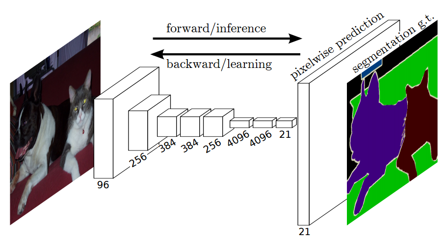 The model basically involves 2 parts: encoder and decoder which can be seen from the image. For encoder and decoder, we can use different combination of different models.
The code to implement the segmentation head is as below
class SegmentationHead(nn.Module):
    def __init__(self, input_channels, num_labels):
        super().__init__()

        self.upconv = nn.Sequential(
            nn.ConvTranspose2d(input_channels,256,3,2,1,1),
            nn.BatchNorm2d(256),
            nn.ReLU(True),
            nn.ConvTranspose2d(256,128,3,2,1,1),
            nn.BatchNorm2d(128),
            nn.ReLU(True),
            nn.ConvTranspose2d(128,64,3,2,1,1),
            nn.BatchNorm2d(64),
            nn.ReLU(True),
            nn.Conv2d(64,num_labels,1,1,0),
        )

    def forward(self, x):
        return self.upconv(x)
The image shown above is from the built-in functionality of Carla simulator. After training the model, the segmentation result will look like the image below.
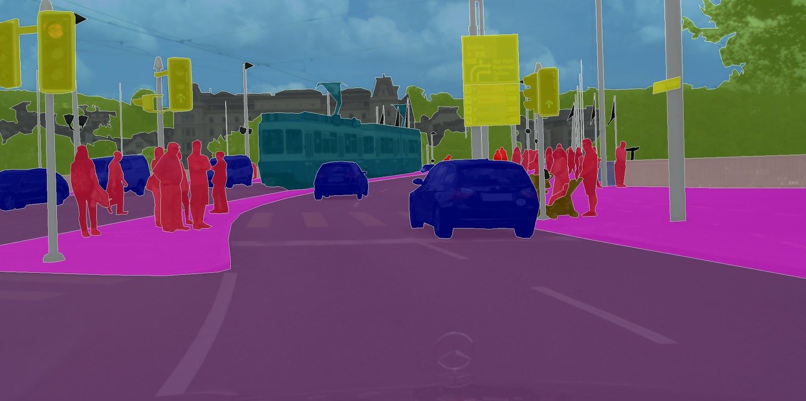 As this is a vision based agent model, the output of the semantic segmentation result cannot be used directly as the input to the action prediction model. But it can help us generate extra loss to meature how good the model learns about the environment.
Innovation
As we have learned from class that there are multiple ways to perform segmantic segmentation. We chose to use one of the modesl proposed in https://github.com/CSAILVision/semantic-segmentation-pytorch. We tried different models proposed in the github repo. In the origional author’s paper, a ResNet34 is used as the backbone model. Therefore, as the encoder, we tried ResNet18, ResNet50 to compute the image features. And as the decoder part, we tried UPerNet and a few other models found in the github repo. Here we post the UPerNet for reference
class UPerNet(nn.Module):
    def __init__(self, num_class=150, fc_dim=4096,
                 use_softmax=False, pool_scales=(1, 2, 3, 6),
                 fpn_inplanes=(256, 512, 1024, 2048), fpn_dim=256):
        super(UPerNet, self).__init__()
        self.use_softmax = use_softmax

        # PPM Module
        self.ppm_pooling = []
        self.ppm_conv = []

        for scale in pool_scales:
            self.ppm_pooling.append(nn.AdaptiveAvgPool2d(scale))
            self.ppm_conv.append(nn.Sequential(
                nn.Conv2d(fc_dim, 512, kernel_size=1, bias=False),
                BatchNorm2d(512),
                nn.ReLU(inplace=True)
            ))
        self.ppm_pooling = nn.ModuleList(self.ppm_pooling)
        self.ppm_conv = nn.ModuleList(self.ppm_conv)
        self.ppm_last_conv = conv3x3_bn_relu(fc_dim + len(pool_scales)*512, fpn_dim, 1)

        # FPN Module
        self.fpn_in = []
        for fpn_inplane in fpn_inplanes[:-1]:   # skip the top layer
            self.fpn_in.append(nn.Sequential(
                nn.Conv2d(fpn_inplane, fpn_dim, kernel_size=1, bias=False),
                BatchNorm2d(fpn_dim),
                nn.ReLU(inplace=True)
            ))
        self.fpn_in = nn.ModuleList(self.fpn_in)

        self.fpn_out = []
        for i in range(len(fpn_inplanes) - 1):  # skip the top layer
            self.fpn_out.append(nn.Sequential(
                conv3x3_bn_relu(fpn_dim, fpn_dim, 1),
            ))
        self.fpn_out = nn.ModuleList(self.fpn_out)

        self.conv_last = nn.Sequential(
            conv3x3_bn_relu(len(fpn_inplanes) * fpn_dim, fpn_dim, 1),
            nn.Conv2d(fpn_dim, num_class, kernel_size=1)
        )

    def forward(self, conv_out, segSize=None):
        conv5 = conv_out[-1]

        input_size = conv5.size()
        ppm_out = [conv5]
        for pool_scale, pool_conv in zip(self.ppm_pooling, self.ppm_conv):
            ppm_out.append(pool_conv(nn.functional.interpolate(
                pool_scale(conv5),
                (input_size[2], input_size[3]),
                mode='bilinear', align_corners=False)))
        ppm_out = torch.cat(ppm_out, 1)
        f = self.ppm_last_conv(ppm_out)

        fpn_feature_list = [f]
        for i in reversed(range(len(conv_out) - 1)):
            conv_x = conv_out[i]
            conv_x = self.fpn_in[i](conv_x) # lateral branch

            f = nn.functional.interpolate(
                f, size=conv_x.size()[2:], mode='bilinear', align_corners=False) # top-down branch
            f = conv_x + f

            fpn_feature_list.append(self.fpn_out[i](f))

        fpn_feature_list.reverse() # [P2 - P5]
        output_size = fpn_feature_list[0].size()[2:]
        fusion_list = [fpn_feature_list[0]]
        for i in range(1, len(fpn_feature_list)):
            fusion_list.append(nn.functional.interpolate(
                fpn_feature_list[i],
                output_size,
                mode='bilinear', align_corners=False))
        fusion_out = torch.cat(fusion_list, 1)
        x = self.conv_last(fusion_out)

        if self.use_softmax:  # is True during inference
            x = nn.functional.interpolate(
                x, size=segSize, mode='bilinear', align_corners=False)
            x = nn.functional.softmax(x, dim=1)
            return x

        x = nn.functional.log_softmax(x, dim=1)

        return x
Reward Design
The reward function \(r(L_t^{ego}, L_t^{world}, a_t, c_t)\) considers ego-vehicle state, world state, action and high-level command, and is computed from the driving log at each timestep. The agent receives a reward of +1 for staying in the target lane at the desired position, orientation and speed, and is smoothly penalized for deviating from the lane down to a value of 0. If the agent is located at a “zero-speed” region(e.g. red light, or close to other traffic participants), it is rewarded for zero velocity regardless of orientation, and penalized otherwise except for red light zones. All “zero speed” rewards are scaled by \(r_{stop} = 0.01\), in order to avoid agents disregarding the target lane.
The agents receives a greedy reward of \(r_{brake} = +5\) if it breaks in the zero-speed zone. To avoid agents chasing braking region, the braking reward cannot be accumulated. All rewards are additive. One interesting observation is that with zero-speed zones and brake rewards, there is no need to explicitly penalize collisions. We compute the action-values over all high-level commands(“turn left”, “turn right”, “go straight”, “follow lane”, “change left” or “change right”) for each timestep, and use multi-branch supervision when distilling the visuomotor agent.
Model Performance
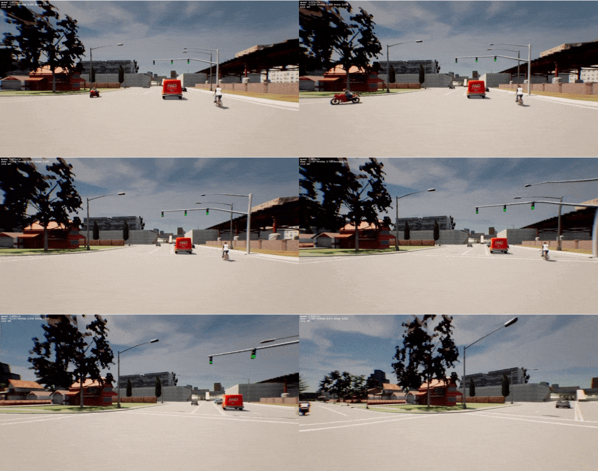
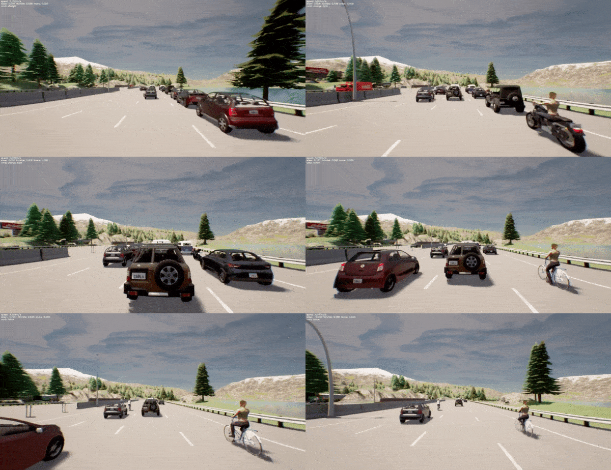
This is how the model performs under the regular condition
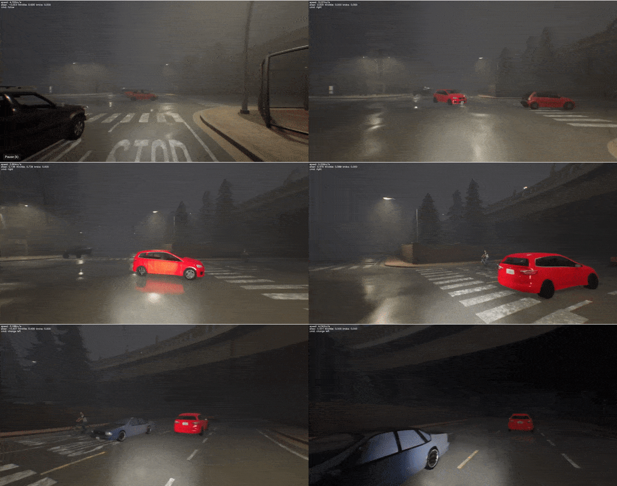
This is how the model performs under rainy condition
This is how the model performs under heady traffic
Reference
[1] Chen, Koltun, et al. “Learning to drive from a world on rails” Proceedings of the International Conference on Computer Vision. 2021.
[2] Dian Chen, Brady Zhou, Vladlen Koltun, and Philipp Kr¨ahenb¨uhl. Learning by cheating. In CoRL, 2019.
[3] Mayank Bansal, Alex Krizhevsky, and Abhijit Ogale. Chauffeurnet: Learning to drive by imitating the best and synthesizing the worst. In RSS, 2019.
[4] B. Zhou, H. Zhao, X. Puig, T. Xiao, S. Fidler, A. Barriuso and A. Torralba. :Semantic Understanding of Scenes through ADE20K Dataset. International Journal on Computer Vision (IJCV), 2018
Code Repository
[1] Learning to drive from a world on rails
[3] ChauffeurNet: Learning to Drive by Imitating the Best and Synthesizing the Worst
[4] CARLA: An Open Urban Driving Simulator
