Semantic Image Editing
Image generation has the potential to greatly streamline creative processes for professional artists. While current capabilities of image generators have shown to be impressive, these models aren’t able to produce good results without fail. However, slightly tweaking text prompts can often result in wildly different images. Semantic image editing has the potential to alleviate this problem, by letting users of image generation models to slightly tweak results in order to achieve higher quality end results. This project will explore and compare some technologies currently available for semantic image editing.
- Semantic Guidance (SEGA)
- Contrastive Language-Image Pre-training (CLIP)
- Cross-Attention Control (Prompt-to-Prompt)
- Demos
- Model Comparisons
- Three Relevant Research Papers
- Reference
If the embed for the video doesn’t work, click here
Semantic Guidance (SEGA)
One option for semantic image editing is semantic guidance. This method bases its functionality on the idea that operations performed in semantic space can result in predictable semantic modifications in the final generated image. A well known example of this can be seen in language prediction: under the word2vec text embedding, the vector representation of ‘King - male + female’ results in ‘Queen’.
Guided Diffusion
SEGA is built upon diffusion for image generation. In diffusion for text-to-image generation, the model is conditioned on a text prompt, and iteratively denoises a Gaussian distribution towards an image that accurately reflects the prompt. Under guided diffusion, this process is influenced in order to “guide” the diffusion in specific directions. This method comes with several advantages over other semantic editors, in that it requires no additional training, no architecture extensions, and no external guidance. In particular, the training objective of a diffusion model \(\hat{x}\) is:
\[\mathbb{E}_{x,c_p,\epsilon,t}[\omega_t \parallel \hat{x}_\theta(\alpha_t x + \omega_t \epsilon, c_p) - x \parallel^2_2]\]Where \((x, c_p)\) is conditioned on text prompt \(p\), \(t\) is sampled from uniform distribution \(t \sim \mathcal{U}([0,1])\), \(\epsilon\) is sampled from Gaussian distribution \(\epsilon \sim \mathcal{N}(0,I)\), and \(\omega_t,\alpha_t\) influence image fidelity based on \(t\). The model is trained to denoise \(z_t := x + \epsilon\), yielding \(x\) with squared error loss.
Additionally, classifier-free guidance is used for conditioning, resulting in score estimates for the predicted \(x\) such that:
\[\tilde{\epsilon}_\theta := \epsilon_\theta(z_t) + s_g(\epsilon_\theta(z_t, c_p) - \epsilon_\theta(z_t))\]where \(s_g\) scales the extent of adjustment, and \(\epsilon_\theta\) defines the noise estimates with parameters \(\theta\).
During inference, the model is sampled using \(x = (z_t - \tilde{\epsilon}_\theta)\)
At a high level, guided diffusion can be explained from the following figure, illustrating the \(\epsilon\)-space (\(\epsilon \sim \mathcal{N}(0,I)\)) during diffusion, and the semantic spaces for the concepts involved in editing a prompt “a portrait of a king”.
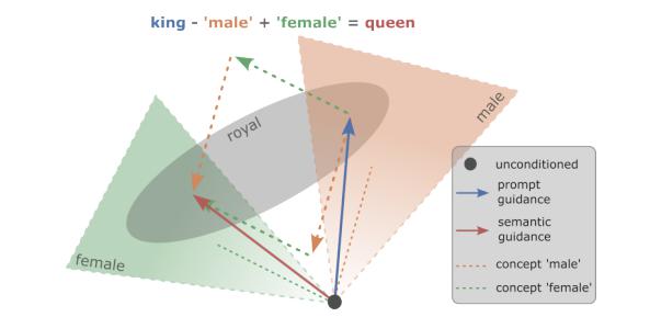
Fig 1. Semantic space under semantic guidance applied to an image with description “a portrait of a king” [2].
Here, the unconditioned noise estimate is represented by a black dot, which starts at a random point without semantic grounding. On executing the prompt “a portrait of a king”, the black dot is guided (blue vector) to the space intersecting the concepts ‘royal’ and ‘male’, resulting in an image of a king. Under guided diffusion, vectors representing the concepts ‘male’ and ‘female’ (orange/green vectors) can be made using estimates conditioned on the respective prompts. After subtracting ‘male’ and adding ‘female’ to the guidance, the black dot arrives at a point in the space intersecting the concepts ‘royal’ and ‘female’, resulting in an image of a queen.
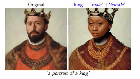
Fig 2. Result of guidance operation using ‘king’ - ‘male’ + ‘female’ [2].
Semantic isolation
A noise estimate \(\epsilon_\theta(z_t, c_e)\) is calculated, conditioned on description \(e\). We calculate the difference between this, and the unconditioned estimate \(\epsilon_\theta(z_t)\), and scale the difference. The numerical values of the resulting latent vector are Gaussian distributed, and the dimensions in the upper and lower tail of the distribution encode the target concept. 1-5% of these dimensions is sufficient to correctly modify the image. Additionally, these concept vectors can be applied simultaneously.
Guidance in a single direction (single concept)
For understanding, we can examine guidance in a single direction, in order to build understanding for guidance in multiple directions. Here, three \(\epsilon\)-predictions are used to move the unconditioned score estimate \(\epsilon_\theta(z_t)\) towards the prompt conditioned estimate \(\epsilon_\theta(z_t, c_p)\) and away/towards the concept conditioned estimate \(\epsilon_\theta(z_t, c_p)\):
\[\epsilon_\theta(z_t) + s_g(\epsilon_\theta(z_t, c_p) - \epsilon_\theta(z_t)) + \gamma(z_t, c_e)\]Here, the semantic guidance term (\(\gamma\)) is defined as
\[\gamma(z_t, c_e) = \mu(\psi;s_e, \lambda)\psi(z_t,c_e)\]where \(\psi\) is defined by the editing direction:
\[\psi(z_t, c_p, c_e) = \begin{cases} \epsilon_\theta(z_t, c_e) - \epsilon_\theta(z_t) & \text{if positive guidance} \\ -(\epsilon_\theta(z_t, c_e) - \epsilon_\theta(z_t)) & \text{if negative guidance} \end{cases}\]and \(\mu\) applies the editing guidance scale \(s_e\) element-wise, and sets values outside of a percentile threshold \(\lambda\) to 0:
\(\mu(\psi;s_e, \lambda) = \begin{cases} s_e & \text{where} |\psi| \geq \eta_\lambda (|\psi|)\\ 0 & \text{otherwise} \end{cases}\) (Here, \(\eta_\lambda(\psi)\) is the \(\lambda\)-th percentile of \(\psi\))
Additionally, SEGA uses two additional adjustments:
- a warm-up parameter \(\delta\) to only apply guidance after a warm-up period \((\gamma(z_t, c_p, c_s) := 0\) if \(t < \delta)\)
- a momentum term \(\nu\) to accelerate guidance after iterations where guidance occurred in the same direction. Finally, we have:
with momentum scale \(s_m \in [0,1]\) and \(\nu\) updated as \(\nu_t+1 = \beta_m \nu_t + (1 - \beta_m) \gamma_t\)
Guidance in multiple directions (multiple concepts)
For each concept \(e_i\), \(\gamma^i_t\) is calculated with its own hyperparameter values \(\lambda^i, s^i_e\). To incorporate multiple concepts, we will take the weighted sum of all \(\gamma^i_t\):
\[\hat{\gamma_t}(z_t,c_p;e) = \sum_{i\in I}g_i \gamma^i_t(z_t, c_p, c_{e_i})\]Each \(\gamma^i_t\) may have its own warm-up period. Hence, \(g_i\) is defined as \(g_i = 0\) if \(t < \delta_i\). Unlike warm-up period, momentum is calculated using all concepts, and applied once all warm-up periods are completed.
Contrastive Language-Image Pre-training (CLIP)
Another option for semantic image editing is contrastive language-image pre-training (CLIP). This method combines the natural language processing approach of CLIP with the semantic image editing of StyleGAN to develop a text-based interface for editing images. This implementation also has the advantage of being able to run on a single commodity GPU instead of research-grade GPU’s.
Latent Optimization
The first approach presented by StyleCLIP is latent code optimization. Given a source latent code \(w_{s} \in \mathcal{W}+\), and a text prompt \(t\), StyleCLIP solves the following optimization problem:
\[\underset{w_{s}\in \mathcal{W}+}{\text{arg min }} D_{\text{CLIP}}(G(w),t) + \lambda_{\text{L2}} \lVert w-w_{s} \rVert_{2} + \lambda_{\text{ID}}\mathcal{L}_{\text{ID}}(w)\]where \(G\) is a pretrained StyleGAN generator and \(D_{\text{CLIP}}\) is the cosine distance between the CLIP embeddings of its two arguments. Similarity to the input image is controlled by the \(L_{2}\) distance in latent space, and by the identity loss:
\[\mathcal{L}_{\text{ID}}(w)=1-\langle R(G(w_{s})),R(G(w))\rangle\]where R is a pretrained ArcFace network for face recognition, and \(\langle.,.\rangle\) computes the cosine similarity between its arguments. StyleCLIP solves this optimization problem through gradient descent, by back-propagating the gradient objective through the pretrained and fixed StyleGAN generator G and the CLIP image encoder.
Latent Mapper
Although latent optimization is effective, it takes several minutes to edit a single image. The second approach presented by StyleCLIP is the use of a mapping network that is trained, for a specific text prompt \(t\), to infer a manipulation step \(M_{t}(w)\) in the \(\mathcal{W}+\) space, for any given latent image embedding \(w \in \mathcal{W}+\).
This latent mapper makes use of three fully-connected networks that feed into 3 groups of StyleGAN layers (coarse, medium, and fine). Denoting the latent code of the input image as \(w=(w_{c},w_{m},w_{f})\), the mapper is defined by
\[M_{t}(w) = (M_{t}^c(w_{c}), M_{t}^m(w_{m}), M_{f}^c(w_{f}))\]The CLIP loss, \(\mathcal{L}_{\text{CLIP}}(w)\), guides the mapper to minimize the cosine distance in the CLIP latent space:
\[\mathcal{L}_{\text{CLIP}}(w) = \mathcal{D}_{\text{CLIP}}(G(w + M_{t}(w), t))\]where \(G\) denotes the pretrained StyleGAN generator. To preserve the visual attributes of the original input image, StyleCLIP minimizes the \(L_{2}\) norm of the manipulation step in the latent space. Finally, for edits that require identity preservation, StyleCLIP uses the identity loss \(\mathcal{L}_{ID}(w)\) defined earlier. The total loss function is a weighted combination of these losses:
\[\mathcal{L}(w) = \mathcal{L}_{\text{CLIP}}(w) + \lambda_{L2} \lVert M_{t}(w) \rVert_{2} + \lambda_{\text{ID}}\mathcal{L}_{\text{ID}}(w)\]
Fig 3. The architecture of the latent mapper using the text prompt “surprised”. First, source image on the left is inverted into a latent code \(w\). Next, three mapping functions are trained to generate residuals which are added to $w$ to yield the target code. Finally, a pretrained StyleGAN generates the modified image [3].
Global Directions
While the latent mapper allows for a fast inference time, the authors found that it sometimes fell short when a fine-grained disentangled manipulation was desired. In addition, the directions of different manipulation steps for a given text prompt tended to be similar. Because of these observations, the third approach presented by StyleCLIP is a method for mapping a text prompt into a single, global direction in StyleGAN’s style space \(\mathcal{S}\), which has been shown to be more disentangled than other latent spaces.
The high-level idea of this approach is to first use the CLIP text encoder to obtain a vector \(\Delta t\) in CLIP’s joint language-image embedding and then map this vector into a manipulation direction \(\Delta s\) in \(\mathcal{S}\). A stable \(\Delta t\) is obtained from natural language using prompt engineering. The corresponding direction \(\Delta s\) is then determined by assessing the relevance of each style channel to the target attribute.
Method Comparison

Fig 4. Comparison between the three methods put forward by StyleCLIP. Notice that although the latent mapper and global direction methods require more time before image generation, the generation process itself is much faster compared to latent optimization [3].
Cross-Attention Control (Prompt-to-Prompt)
The final option we will explore for semantic image editing is cross-attention control. This approach uses cross-attention maps, which are high-dimensional tensors that bind pixels and tokens extracted from the prompt text. These maps contain rich semantic relations which affect the generated image.

Fig 5. A visual representation of the processes described below [1].
Cross-Attention in Text-Conditioned Diffusion Models
In a diffusion model, each diffusion step \(t\) consists of predicting the noise \(\epsilon\) from a noisy image \(z_{t}\) and text embedding \(\psi(\mathcal{P})\) using a U-shaped network. The final step yields the generated image \(\mathcal{I}=z_{0}\). More formally, the deep spatial features of the noisy image \(\phi (z_{t})\) are projected to a query matrix \(Q = \ell_{Q}(\phi(z_{t}))\), and the textual embedding is projected to a key matrix \(K = \ell_{K}(\psi(\mathcal{P}))\) and a value matrix \(V = \ell_{V}(\psi(\mathcal{P}))\), via learned linear projections \(\ell_{Q}\), \(\ell_{K}\), and \(\ell_{V}\). Attention maps are then
\(M = \text{Softmax}(\frac{QK^{T}}{\sqrt{d}})\), where the cell \(M_{ij}\) defines the weight of the value of the \(j\)-th token on the pixel \(i\), and \(d\) is the latent projection dimension of the keys and queries. Finally, the cross-attention output is defined to be \(\hat{\phi}(z_{t}) = MV\), which is then used to update the spatial features \(\phi(z_{t})\).
Intuitively, the cross-attention output \(MV\) is a weighted average of the values \(V\) where the weights are the attention maps \(M\), which are correlated to the similarity between \(Q\) and \(K\).
Controlling the Cross-Attention
Pixels in the cross-attention maps are more attracted to the words that describe them. Since attention reflects the overall composition, injecting the attention maps \(M\) obtained from the generation with the original prompt \(\mathcal{P}\) into a second generation with the modified prompt \(\mathcal{P}^{*}\) allows the synthesis of an edited image \(\mathcal{I}^{*}\) that is manipulated according to the edited prompt while keeping the structure of the original image \(\mathcal{I}\) intact.

Fig 6. Visualizations of cross-attention maps. The top row shows the average attention masks for each word in the prompt for the image on the left. The bottom row shows the attention maps for with respect to the word “bear” across different time-stamps [1].
Let \(DM(z_{t}, \mathcal{P}, t, s)\) be the computation of a single step in the diffusion process which outputs the noisy image \(z_{t-1}\) and the attention map \(M_{t}\). Let \(DM(z_{t}, \mathcal{P}, t, s) \lbrace M \gets \widehat{M} \rbrace\) be the diffusion step where the attention map \(M\) is overridden with an additional given map \(\widehat{M}\) with the same values \(V\) from the supplied prompt. Let \(M_{t}^{*}\) be the produced attention map from the edited prompt \(\mathcal{P}^{*}\). Let \(Edit(M_{t}, M_{t}^{*}, t)\) be a general edit function that receives the \(t\)-th attention maps of the original and edited images as input.
The general algorithm for controlled generation performs the iterative diffusion process for both prompts simultaneously, where an attention-based manipulation is applied in each step according to the desired editing task. The internal randomness is fixed since different seeds produce wildly different outputs, even for the same prompt.
Algorithm 1: Prompt-to-Prompt Image Editing
Input: A source prompt \(\mathcal{P}\), a target prompt \(\mathcal{P}^{*}\), and a random seed \(s\)
Optional for local editing: \(w\) and \(w^{*}\), words in \(\mathcal{P}\) and \(\mathcal{P}^{*}\), specifying the editing region
Output: A source image \(x_{src}\) and an edited image \(x_{dst}\)
\(z_{T} \sim N(0, I)\) A unit Gaussian random variable with random seed \(s;\)
\(z_{T}^{*} \gets z_{T};\)
for \(t = T, T-1, ..., 1\) do
\(z_{t-1}, M_{t} \gets DM(z_{t}, \mathcal{P}, t, s);\)
\(M_{t}^{*} \gets DM(z_{t}^{*}, \mathcal{P}_{t}^{*}, t, s);\)
\(\widehat{M}_{t} \gets Edit(M_{t}, M_{t}^{*}, t);\)
\(z_{t-1}^{*} \gets DM(z_{t}^{*}, \mathcal{P}^{*}, t, s) \lbrace M \gets \widehat{M}_{t} \rbrace\)
if \(local\) then
\(\alpha \gets B(\overline{M}_{t, w}) \cup B(\overline{M}_{t, w^{*}}^{*});\)
\(z_{t-1}^{*} \gets (1 - \alpha) \odot z_{t-1} + \alpha \odot z_{t-1}^{*}\)
end
end
Return \((z_{0}, z_{0}^{*})\)
Local Editing
To modify a specific object or region while leaving the rest of the scene intact, the cross-attention map layers corresponding to the edited object are used. A mask of the edited part is approximated and the modification is constrained to be applied only in this local region. To calculate the mask at step \(t\), compute the average attention map \(\overline{M}_{t, w}\) (averaged over the steps \(T,...,t\)) of the original word \(w\) and the map \(\overline{M}_{t, w^{*}}^{*}\) of the new word \(w^{*}\). Next, apply a threshold to produce binary maps (\(B(x) := x > k\) and \(k = 0.3\)). The final mask \(\alpha\) is a union of the binary maps since the edited region should include silhouettes of both the original and the newly edited object to support geometric modifications. Finally, the mask is used to constrain the editing region, where \(\odot\) denotes element-wise multiplication.
Word Swap
“Word swap” is the case where the user swaps tokens in the prompt with alternatives, such as \(\mathcal{P} =\) “a big bicycle” and \(\mathcal{P}^{*} =\) “a big car”. In order to preserve the original composition while addressing the content of the new prompt, the attention maps of the source image are injected into the generation with the modified prompt. Since this attention injection may over-constrain the geometry, a softer attention constrain is used: \(Edit(M_{t}, M_{t}^{*}) := \begin{cases} M_{t}^{*} & \text{if } t < \tau \\ M_{t} & \text{otherwise.} \end{cases}\)
where \(\tau\) is a timestamp parameter that determines until which step the injection is applied. Since the composition is determined in the early steps, by limiting the number of injection steps, the composition will have the necessary geometric freedom for adapting to the new prompt. Another relaxation is to assign a different number of injection steps for different tokens in the prompt. If two words are represented using a different number of tokens, the maps are duplicated/averaged as necessary using an alignment function described next.
Prompt Refinement
“Prompt refinement” is the case where a user adds new tokens to the prompt, such as \(\mathcal{P} =\) “a castle” and \(\mathcal{P}^{*} =\) “children drawing of a castle”. To preserve the common details, the attention injection is only applied over the common tokens from both prompts. The alignment function \(A\) receives a token index from the target prompt \(\mathcal{P}^{*}\) and outputs the corresponding token index in \(\mathcal{P}\) or \(None\) if there is no match. Then, the editing function is: \(Edit(M_{t}, M_{t}^{*}, t)_{i, j} := \begin{cases} (M_{t}^{*})_{i, j} & \text{if } A(j) = None \\ (M_{t})_{i, A(j)} & \text{otherwise.} \end{cases}\)
where \(i\) coresponds to a pixel while \(j\) corresponds to a text token.
Attention Re-Weighting
Lastly, the user may wish to strenghten or weaken how much each token affects the resulting image. For example, consider the prompt \(\mathcal{P} =\) “a fluffy ball”, and assume the user wants to make the ball more or less fluffy. To achieve this, the attention map of the assigned token \(j^{*}\) is scaled with a parameter \(c \in [-2, 2]\), resulting in a stronger or weaker effect. The rest of the attention maps remain unchanged. Thus, the editing function is: \(Edit(M_{t}, M_{t}^{*}, t)_{i, j} := \begin{cases} c \cdot (M_{t})_{i, j} & \text{if } j = j^{*} \\ (M_{t})_{i, j} & \text{otherwise.} \end{cases}\)
Demos
We have included a colab notebooks demonstrating each of the methods we have examined:
- SEGA
- StyleCLIP (latent optimization)
- StyleCLIP (latent mapper)
- StyleCLIP (global directions)
- Prompt to Prompt
Model Comparisons
In order to compare each of these methods, we initially devised two different studies
- In the first study, we will assess the rate at which models could create “acceptable” inferences
- In the second study, we will assess the overall quality of the outputs, through use of a survey
Experiment 1: Prompt Success Rate
When exploring the models, we noticed that oftentimes models would completely fail to generate acceptable results for specific prompts, even across different seeds. For this experiment, we intended to explore how often each model can successfully generate an image based on a prompt, and possibly find if certain prompts appear to be universally difficult to generate.
One problem we ran into when conducting the experiment was the number of unique hyperparameters for each model. It would have been prohibitively time consuming to test the full range of possible hyperparameter combinations across all models. As a compromise, we fixed the hyperparameters for each model to the hyperparameters that we arrived at when trying to generate the highest possible quality images for the second part of our study (with the exception for training steps, which we set to 50 for models that had this hyperparameter)
Note: StyleCLIP’s latent mapper method was excluded from this portion of the study, due to its architectural specifics. In particular, the latent mappers available to use could only make a very limited set of edits applicable to a small library of celebrity images, and thus comparison to the other four models would have been extremely limited
Procedure
For this experiment, we collected 50 sample points (reseeding the model with a random seed between each sample) from each model on two different prompts
- person -> person with beard
- person -> person with glasses
Note: the way these prompts were applied varied slightly between models, but in general the prompts followed this idea
For each sample point, three people voted on whether the model had acceptably applied the edit (in this case, “acceptably” meant that the model had applied the edit while retaining most of the details from the initial image)
Results
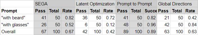
Table 1. Prompt Success Rates.
From these results, we’re able to conclude that prompts are not necessarily “universally difficult” - different models had varying levels of success with different prompts.
While not necessarily part of this study, in developing the experiment we discovered that small differences between prompts can result in massively changed generations (for example, StyleCLIP’s latent optimization method appeared to have slightly better results when processing the grammatically incorrect prompt “a old man” when compared to the prompt “an old man”)
Experiment 2: Generation Quality
For this portion of the study, we intended to gauge the overall quality of generated images. However, we realized that it would be very difficult to obtain objective results, due to the sheer number of variables involved. From our previous study, one main takeaway we had learned was that different models seemed to be better at performing different types of edits. Furthermore, since the models were not trained on the same datasets, different models had inherent advantages for different prompts (for example, the StyleCLIP models, trained on FFHQ, were unable to render anything besides faces, but appeared to be much better at generating human faces than the other models as a result). Regardless, we were curious to see what our friends thought of the power of the models, and so we decided to collect survey results to gauge people’s opinions.
Procedure
For each of the models, we collected the best sample result we could from three prompts:
- “Man with a beard”
- “Man wearing glasses”
- “Man with no hair”
Note: for StyleCLIP’s latent mapper, we simply included three random prompts, for the same reasons as outlined above
Additionally, we included three control images (survey respondents were not told how many of the presented images were real photographs, only that some of them were)
Survey respondents were presented with unlabeled images, and were asked to rate the image on a scale of 1 to 5 on how well the AI did at creating the image.
Results
Initially, we tried to run the survey with more examples, but the first few survey respondents complained about survey length. After reducing the survey size, we obtained the following results from surveying 30 people:
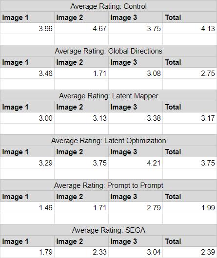
Table 2. Average Rating Per Image/Model.
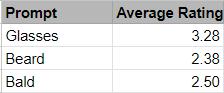
Table 3. Average Rating Per Prompt.
While we tried to fix as many variables as possible when running this survey, the study is clearly not rigorous. Nonetheless, we noted some interesting details:
- The control images performed surprisingly poorly, with some generated examples matching or exceeding the ratings of some real photographs.
- On average, adding glasses was more convincing than adding a beard or removing hair
- StyleCLIP’s Latent Mapper didn’t perform as well as expected, despite being a more focused model and having easier prompts (This was likely due to survey respondent confusion, which lead to respondents rating these images lower due to being able to recognize the images as clearly manipulated)
Additional Comparisons
A more objective comparison that we were able to make in our exploration was per-prompt generation time:

Table 4. Generation Time For One Image.
(For models that used maximum steps as a hyperparameter, this was fixed to 50)
Notably, the methods presented by StyleCLIP are significantly faster than Prompt to Prompt and SEGA. Impressively, the latent mapper and global directions methods are both able to produce results in less than a second each (granted, the latent mapper method is heavily dependent on being able to train a focused mapper, while the global directions method requires twice as much human input as other methods).
Conclusions
As beginners, we found it particularly difficult to set up and use the implementations of the methods we chose to explore. Due to various factors, including outdated libraries, bugs, and incompatible hardware, it took many hours of debugging, research, and trial and error to be able to run our demo notebooks and collect results. In some cases, we had to directly solve some of these problems in code, making forks and manually fixing outdated and broken code. For some projects we initially intended to explore, the hours spent poring over various project repositories went to waste, as we were ultimately unable to find a way to run these methods successfully. Even for the models that we were eventually able to successfully collect results from, we weren’t able to do everything we had planned to do. Ideally, we would have liked to train each of the models from the same datasets in order to offer a more fair and objective comparison, but due to time and resource constraints we ultimately weren’t able to do this. Additionally, we made some naive assumptions in the initial stages of experimentation, and as a result encountered problems with specific prompts for some models, and had to throw away all previously collected data points.
Despite the difficulties we experienced with this project, we nonetheless believe it was a good learning experience (a good example of “trial by fire”). We became much faster at diagnosing technical problems with setting up models after we successfully set up our first two models.
Aside from the technical challenges we faced, we encountered many obstacles in the experimental design process. While some computer vision models, such as classification, have obvious ways to compare and compute performance, we learned that this isn’t necessarily true for all of them. While surveys may seem like an obvious way to gauge the performance of generative models, we learned that it is not always easy to develop an easily understood scale for ordinary people to rate things by. If anything, our struggles to design a sound experiment highlight the difficulties that researchers may face when attempting to compare different models and methods objectively.
Granted a second chance (and more time), we would have liked to make the following key improvements:
- Retrain the models to use the same dataset
- Try a wider variety of prompts, and collected more sample data points
- Collect results for different combinations of hyperparameters
- Obtain more survey responses
In the end, we hope that you have learned something interesting about semantic image editing, and have gained a glimpse into what the future might hold for the technology.
Three Relevant Research Papers
-
Prompt-to-Prompt Image Editing with Cross Attention Control
- [Paper] https://arxiv.org/abs/2208.01626
- [Code] https://github.com/google/prompt-to-prompt
-
SEGA: Instructing Diffusion using Semantic Dimensions
- [Paper] https://arxiv.org/abs/2301.12247
- [Code] https://github.com/ml-research/semantic-image-editing
-
StyleCLIP: Text-Driven Manipulation of StyleGAN Imagery
- [Paper] https://arxiv.org/abs/2103.17249
- [Code] https://github.com/orpatashnik/StyleCLIP
Reference
[1] Hertz, Amir, et al. Prompt-to-Prompt Image Editing with Cross Attention Control. 1, arXiv, 2022, doi:10.48550/arXiv.2208.01626.
[2] Brack, Manuel, et al. SEGA: Instructing Diffusion using Semantic Dimensions. 1, arXiv, 2022, doi:10.48550/arXiv.2301.12247.
[3] Patashnik, Or, et al. StyleCLIP: Text-Driven Manipulation of StyleGAN Imagery. 1, arXiv, 2021, doi:10.48550/arXiv.2103.17249.