Medical Imaging

Medical Imaging analysis has always been a target for the many methods in deep learning to help with diagnostics, evaluations, and quantifying of medical diseases. In this study, we learn and implement models of Logistic Regression and ResNet18 to use in medical image classification. We use image classification to train our models to find brain tumors in brain MRI images. Furthermore, we will use our own implementation of LogisticRegression and finetune our ResNet18 model to better fit our needs.

• Introduction
• Logistic Regression
  • Motivation
  • Architecture
  • Code Implementation
• ResNet18
  • Motivation
  • Architecture
  • Code Implementation
• DenseNet
  • Motivation
  • Architecture
  • Code Implementation
• EffecientNet
  • Motivation
  • Architecture
  • Code Implementation
• Result
• Demo
• Reference

Introduction

We explore different methods of image classification with brain MRI images that may consist of a brain tumor. We train models such as LogisticRegression and ResNet18 and implement them to achieve the best accuracies. The LogisticRegression model was created with our own logic and implementation while the ResNet18 model was finetuned for the task.

Logistic Regression

Motivation

Medical imaging is very important when attempting to document the visual representation of a likely disease. Being able to have a larger sample size can help solidify the accuracy the likelihood of diseases. However, it will take a long time and also allow for human error whenever these images are observed by a human. Therefore, it is important for image classification in medical imaging to be as precise and fast as possible. To address this, we use Logistic Regression as a model to accurately and quickly give us the likelihood of a brain tumor. Logistic Regression is quick whenever the response is binary, hence it is a great model to use for our use case. Some challenges that may occur when implementing our design are:

1. High Dimensionality can cause an image to have a large number of pixels depending on our dataset images which can cause overfitting or slow training.
2. Invariance in our transformations can cause the training model to not take into consideration any images with more variations such as rotated images when image scans are not perfectly straight.
3. Dataset image dependency is huge here because if there are more images in one image class than the other, there can be an imbalance.

Architecture

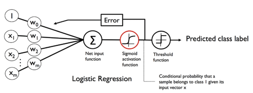
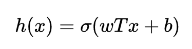
The Logistic Regression model is a relatively simple model compared to other complex models like neural networks. There is a single layer of neurons where each neuron computes the weighted sum of the input features and applies the sigmoid function to the result to produce the probability estimate. We apply the sigmoid function to a the simple Linear Regression equation. It is the sigmoid function that maps the weighted sum inputs to the value between 0 and 1 which is the predicted probability that the input belongs in the right class. The common loss function for the Logisitic Regression model is the cross-entropy loss. This loss function measures the difference between the predicted probability distribution and the true probability distribution.

Code Implementation

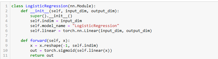
As described previously, our implementation also has the input image passes through a linear layer to calculate a weighted sum of the input features. Then to that output from the linear layer, we apply the sigmoid function in our forward() function. This is the process that maps the weight sum inputs to values between 0 and 1.

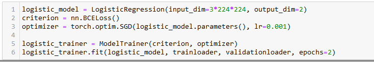
Here we can see that we apply our common loss function where criterion is described. This is where the loss function distributes the predicted probability and ground-truth probabilities.

ResNet18

Motivation

When it comes to image classification and the Logistic Regression model is a very simple yet quick method when the result is binary. However, this does not mean we cannot use more complex neural network architectures for the task. ResNet18 is a deep neural network architecture that is designed for image classification and is a variant of the ResNet architecture that uses 18 layers including a convolutional layer, four residual blocks, and a fully connected layer. With the introduction to these residual blocks, it removes the vanishing gradient problem because as each layer calculates the gradient layer, it can become exponentially small as our input propagates through each layer. Some reasons why we want to use the ResNet18 model against our Logistic Regression are,

1. Feature extraction in ResNet18 compared to Logistic Regression's manual feature extraction, can learn hierarchical features from the input image and we want to know how that compares to Logistic Regression.
2. ResNet18 can also handle more noisy and complex input images compared to Logistic Regression since we can use the multiple layers to extract features.
3. Performance is the final difference we want to test when compared to Logistic Regression as ResNet18 has previously reached many amazing benchmarks in image classification.

Architecture

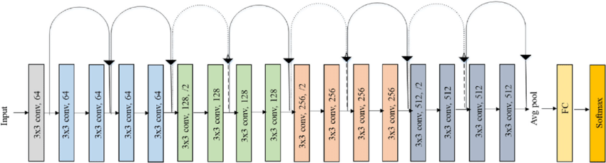
ResNet18 uses 18 layers residual blocks compared to other neural networks to avoid the vanishing gradient problem. The input changes each layer due the convolutional layers and pooling that occurs during the process. Each convolutional layer is followed by a batch normalization layer and a ReLu activation function. These layers contain four stages which each stage consisting of the residual blocks. Each of these residual blocks contain some convolutional layers with shortcut connections that allow the prevention of the vanishing gradient problem.

The first convolution layer is the raw input data represented by a 3D vector which is then output with another 3D vector but with a different number of channels. Subsequent layers continue this procedure using the last layer’s output as the next layer’s input followed by the batch normalization and ReLu activation function. The avgpool layer reduces the height and width of our image classification without changing the number of channels. This helps reduce the spatial dimensions of a feature map while keeping the most important features of our MRI images. The FC layer or fully connected layer, connects every neuron in the previous layer to every neuron in the current layer. For our use case, we use it to map the output of the previous layer to our class labels.

Code Implementation

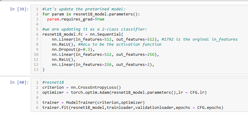
Using the timm library, we implement the ResNet18 model as we did for our assignment in class. The model itself contains the expected layers and activation functions required. Similar to how we implemented it in class, we did change the final classification layer to fit out dataset for image classification.

DenseNet

Motivation

In comparison to the models we previously worked with, we did some research on other image classification models that can be compared to Logistic Regression and Resnet18 that may provide improved accuracy. DenseNet was one of these model we decided to implement. Through our research of the model and its capabilities, we can expect:

1. DenseNet's dense connectivity pattern allows the model to reuse features and improves gradient flow between layers for better feature learning and classification.
2. DenseNet's connectivity pattern to also reduce overfitting compared to that of Logistic Regression and ResNet18.
3. A reduced vanishing gradient with DenseNet compared to the previous two models because DenseNet allows gradients to flow directly from one layer to another without having to pass through multiple non-linear transformations.

Architecture

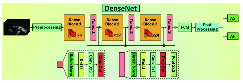
The DenseNet architecture can be summarized as follows, input, initial convolutional layer, dense blocks, transition layers, global average pooling, and finally the output.

A Dense Block is a group of layers that are ‘densely’ connected to each other. This dense connectivity pattern connects each layer to all previous layers in the block. In other words, we can expect that all output feature maps from each layer of a Dense Block are combined with the feature maps from all previous layers in the same block. These layers are then passed to the next block. This is what allows DenseNet to enable feature reuse and improves gradient flow. Lastly, this also reduces the number of parameters required to achieve high accuracies.

Transition layers are also another unique feature of the DenseNet model. Transition layers are used between a pair of dense blocks to reduce the number of feature maps and spatial resolutions. The transition layers are responsible for keeping computational costs low as well as keeping the number of parameters controlled. Typically, a transitional layer is a 1x1 convolutional layer that is followed by a average pooling layer to reduce both the number of feature maps and spatial resolution. Transition layers are one of the key components that allows DenseNet to keep its unique feature of keeping parameters low.

Lastly, after the final dense block has been passed, the output feature maps pass through a global average pooling layer to reduce its spatial dimensions to a single value per map. This output is then passed through a fully connected layer and a activation function.

Code Implementation

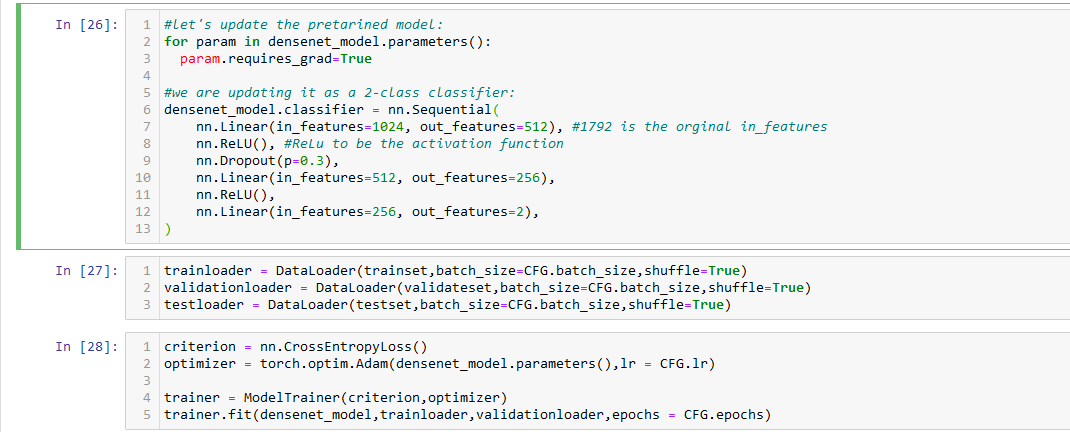
Similar to ResNet18, we used the timm library to implement the DenseNet model as well. Looking through the model, it behaves as the architecture described. It uses a combination of multiple dense blocks and transition layers to form a densely formed network. The input is passed through these blocks and layers and finally globally average pooled. Here we also describe the multiple DataLoaders and use CrossEntropyLoss for our loss function.

EffecientNet

Motivation

EffecientNet tries to achieve state-of-the-art performance by minimizing parameters and maintaining low performance cost. The way EffecientNet achieves this is by utilizing an approach called “compound scaling”. Compound Scaling involves scaling the network in a balanced way. Depth, width, and resolution is increased respectively by adding more layers or adding more filters. The resolution is increases as well to improve the quality of features learned. EffecientNet was the last of our models to use for comparison because of the performance and accuracy it boasts during our research.

Architecture

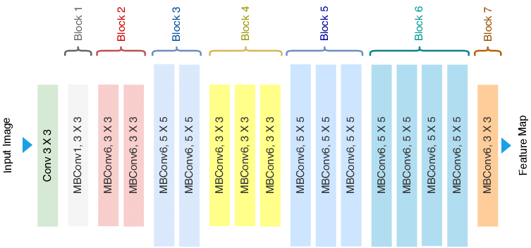
EffecientNet’s architecture comprises of the input image going through a series of convolutional layers to reduce its spatial dimension and increase its depth. The first block contains multiple MBConv blocks with each block consisting of a depthwise convolution, a pointwise convolution, and a squeeze-and-excitation module (SE module). After the input image goes through the sequence of MBConv blocks, it is passed to a Average Pooling layer which then computes the average feature map over its spatial dimensions. This produces a feature vector that is passed to a fully connected layer to produce the final classification results.

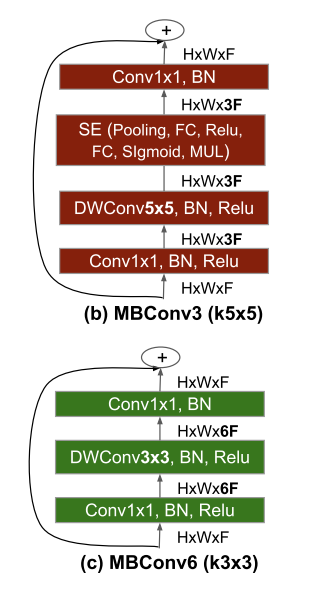
The MBConv block is what makes EffecientNet do what it can and it works by running through some different types of convolutions. The three main operations that take place are,

1. Depthwise convolution where the input has a separate convolutional filter appleid to each channel of the input. This process helps the model reduce computing costs since it applies fewer filters than a regular convolution.
2. Pointwise convolution then takes the output of the depthwise convolution where it applies a 1x1 convolutional filter. This increases the channels of the output which allows the network to learn more complex features.
3. Squeeze-and-Excitation Module then takes the output of the pointwise convolution to find any interdependencies between channels. It does this by using weights to help represent the importance of each channel. This module is very important because it helps the network focus on the most important channels.
4. Residual Connection finally takes the output of the SE Module and is then added to the input of the next MBConv block, creating a residual connection. This is also a very important connection that helps ensure the network learn and identify the most important features. This allows the connection to avoid issues like the vanishing gradient.

Code Implementation

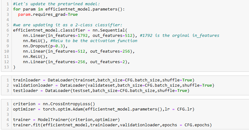
Last of the models that we chose to implement is the EffecientNet. Similar to the last to models, we use the timm library to implement the EffecientNet model. When looking through the model, we saw that the model behaves as expected with the many MBConv blocks forming together. Each of the MBConv blocks have the depthwise convolution, pointwise convolution, and the squeeze-and-excitation modules. Similar to DenseNet, we have a set of DataLoaders and utilizies a CrossEntropyLoss as its loss function.

Result

Logistic Regression 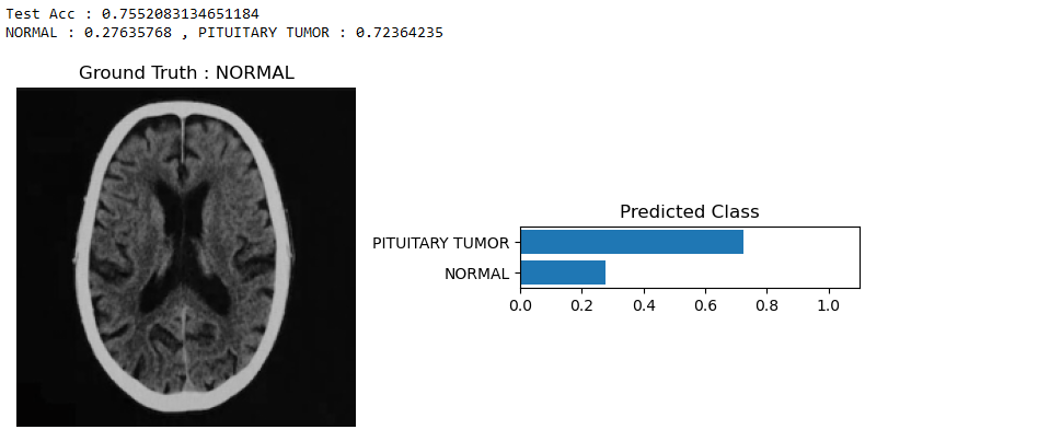The Logistic Regression model was incorrect when making the correct prediction. From the test accuracy, we can see that it is 75%. The ground truth being NORMAL, we can see from the PREDICTED CLASS predicts that there is a tumor.

ResNet18 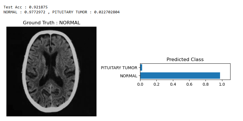ResNet18 performed the best out of all of our models which was a surprise. We knew that ResNet18 performs extremely well with limited datasets but it performed exceptionally well. With a testing accuracy of 92%, the PREDICTED CLASS was very confident when dictating the predicted class. The ground truth being NORMAL, ResNet18 performed above our expectations.

DenseNet 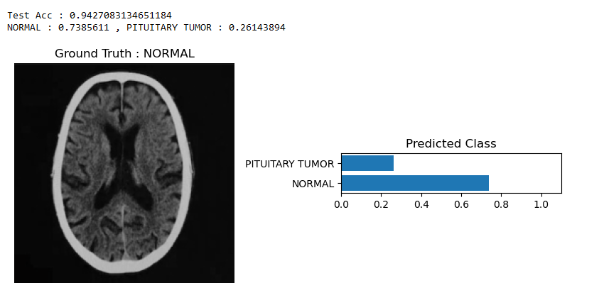DenseNet performed neither too poorly or too exceptionally. With a testing accuracy of 94%, we expected a much more confident prediction when it came to PREDICTED CLASS. However, we do see that the model classified the image correctly, therefore, it performed somewhat as expected.

EffecientNet 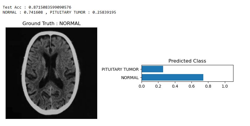Lastly, with EffecientNet, we had very high expectations in this model. However, the interesting observation is that it had a lower testing accuracy than DenseNet. However, the model had a testing accuracy of 87% and the PREDICTED CLASS seemed just as confident as DenseNet. The model predicted the class correctly and this falls under our expectations.

Demo

Video: Here

Code Base: Here

Reference

1. Torres, Renato, et al. ‘A Machine-Learning Approach to Distinguish Passengers and Drivers Reading While Driving’. Sensors, vol. 19, 07 2019, p. 3174, https://doi.org10.3390/s19143174.
2. Ramzan, Farheen, et al. ‘A Deep Learning Approach for Automated Diagnosis and Multi-Class Classification of Alzheimer’s Disease Stages Using Resting-State FMRI and Residual Neural Networks’. Journal of Medical Systems, vol. 44, 12 2019, https://doi.org10.1007/s10916-019-1475-2.
3. Sanagala, Siva Skandha, et al. ‘Ten Fast Transfer Learning Models for Carotid Ultrasound Plaque Tissue Characterization in Augmentation Framework Embedded with Heatmaps for Stroke Risk Stratification’. Diagnostics, vol. 11, Nov. 2021, p. 2109, https://doi.org10.3390/diagnostics11112109.
4. https://iq.opengenus.org/efficientnet/

A collection of recent image segmentation methods, categorized by regions of the human body

A student project from last year in this class. They have specifically studied PDV-Net and ResUNet++.

A review paper discussing the various methods in deep learning used for medical imaging.

A medical imaging toolkit for deep learning.

A paper that focuses on data preparation of medical imaging data for use in machine learning.

Meta analysis of diagnostic accuracy of deep learning methods in medical imaging.

---