Multi View Stereo (MVS)
This post provides an introduction to Multi View Stereo (MVS) and presents to deep learning based algorithms for MVS reconstruction.
- Multi View Stereo (MVS)
- DTU MVS
- TransMVSNet
- CDS-MVSNet
- Comparing TransMVSNet and CDS-MVSNet
- Appendix
- Reference
Multi View Stereo (MVS)
Multi View Stereo (MVS) reconstructs a dense 3D geometry of an object or scene from calibrated 2D images taken from multiple angles. It is an important computer vision task as it is a pivotal step in robotics, augmented/virtual reality, automated navigation and more. Deep learning, with its success in computer vision tasks, has been increasingly used in solving 3D vision problems, including MVS. In this project, we are going to investigate two state-of-the-art MVS frameworks – TransMVSNet that uses a transformer-based deep neural network and CDS-MVSNet, which is a dynamic scale feature extraction network using normal curvature of the image surface.
DTU MVS
The DTU MVS dataset is a publicly available dataset used for evaluating MVS algorithms. It was created by the Technical University of Denmark (DTU) and contains a variety of scenes, each captured from multiple viewpoints. The dataset includes 59 scenes that contain 59 camera positions and 21 that contain 64 camera positions. The scenes vary in geometric complexity, texture, and specularity. Each image is 1200x1600 pixels in 8-bit RGB color.
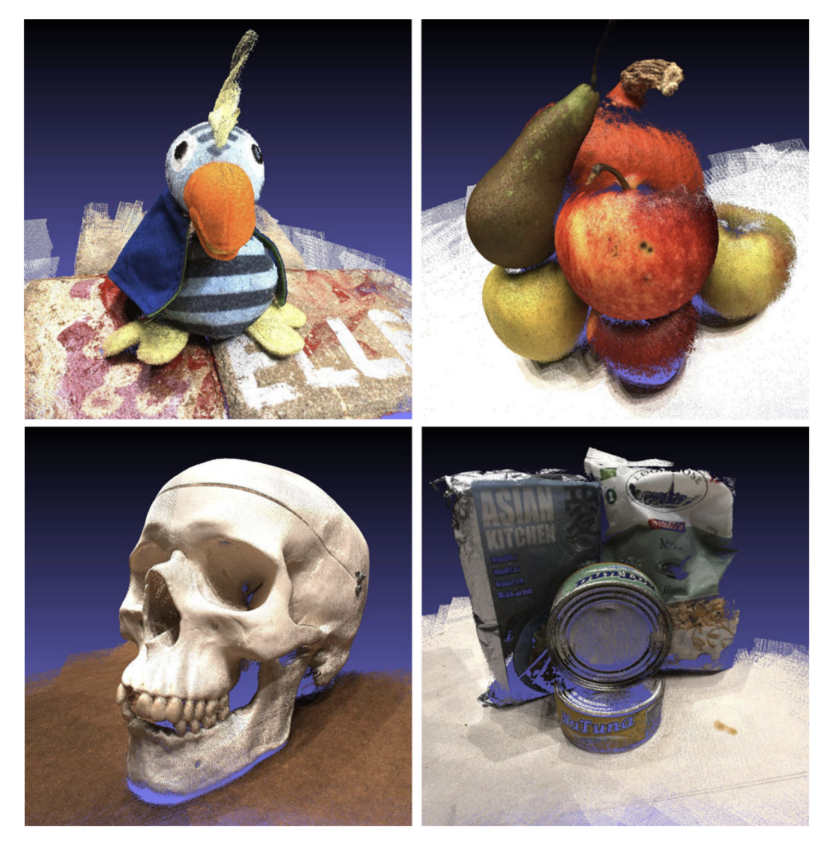
Fig 1. Examples of reference point clouds in DTUMVS dataset. The subset includes scenes of various texture, geometry, and reflectance [1].
The dataset provides reference data (ground truth depth) by measuring a reference scan from each camera position and combining them. The DTU MVS dataset is widely used in the computer vision community as a benchmark for evaluating and comparing different multi-view stereo algorithms. We are going to use this dataset to reproduce and compare the results of the two algorithms that this project focuses on.
TransMVSNet
Motivation
Transformer, originally proposed for natural language processing, has gained increasing popularity in the computer vision community as well. The attention mechanism and positional encoding in transformers allow it to capture global and local information, Multi-view stereo, on the other hand, can be viewed as a one-to-many mapping task, requiring knowledge of information within each image and between two images. Hence, TransMVSNet is proposed to leverage a feature mapping transformer in the MVS task.
Architecture
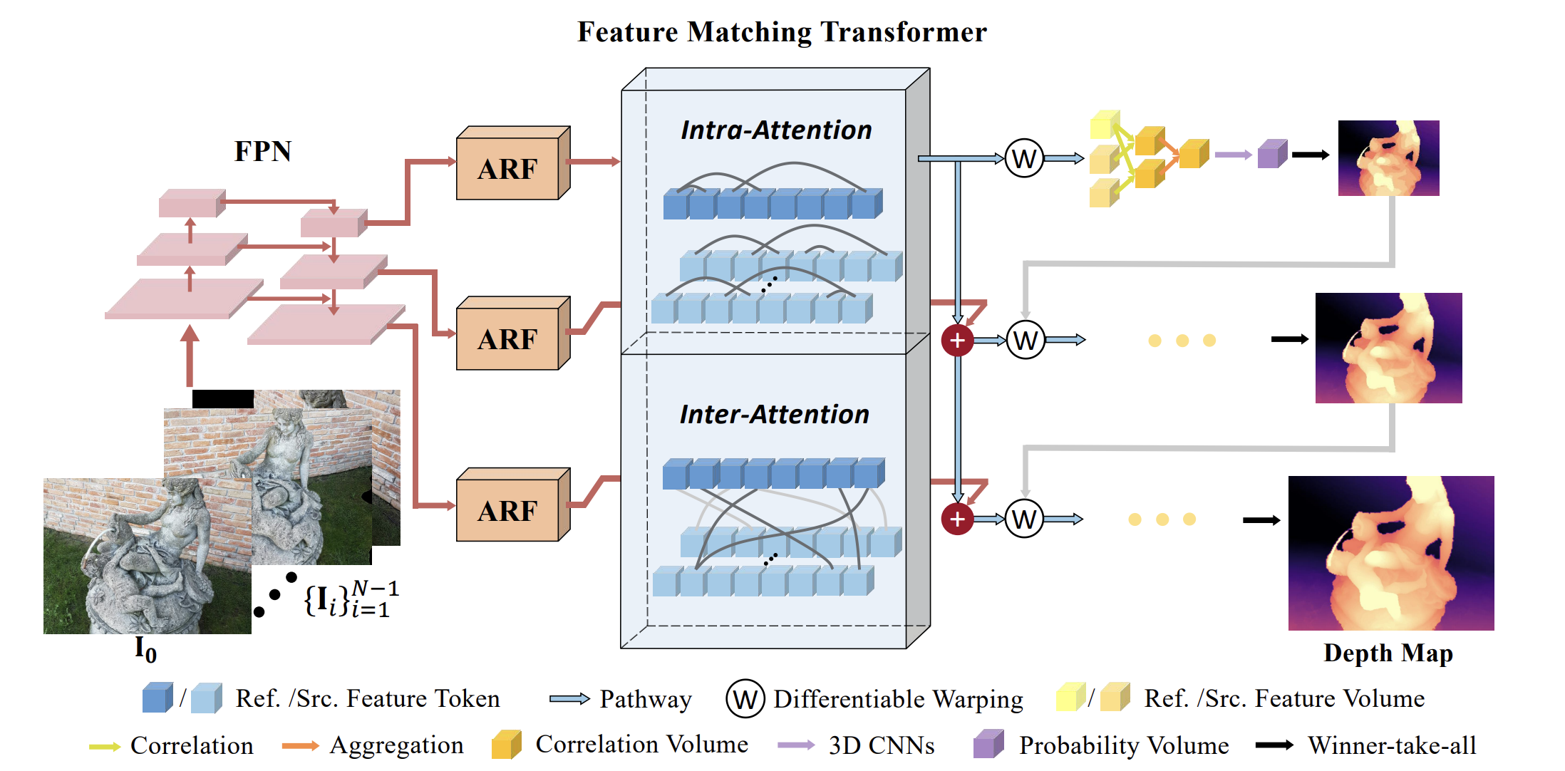
Fig 2. TransMVSNet architecture [1].
TransMVSNet is an end-to-end deep neural network model for MVS reconstruction. Fig. 2 shows the architecture of TransMVSNet. TransMVSNet first applies a Feature Pyramid Network (FPN) to obtain three deep image features with different resolutions. Then, the scope of these extracted features are adaptively adjusted through an Adaptive Receptive Field Module (ARF) that is implemented by deformable convolution with learnable offsets for sampling. The features adjusted to the same resolutions are then fed to the Feature Matching Transformer (FMT). The FMT first performs positional encoding to these features and flattens them. Then, the flattened feature map is fed to a sequence of attention blocks. In each block, all features first compute an intr-attention with shared weights, and then each reference feature is updated with a unidirectional inter-attention information from the source feature. The feature maps processed by FMT then go through a correlation volume and 3D CNNs for regularization to obtain a regularized probability volume. Then, winner-take-all is used to determine the final prediction.
Architecture Blocks and Code Implementation
Given a reference image \(I_0\in \mathbb{R}^{H\times W\times 3}\) and its neighboring images \(\{I_i\}_{i=1}^{N-1}\), as well as their respective camera intrinsics and extrinsics, the aim of this model is to predict a depth map aligned with the reference image \(I_0\) and to filter and use all depth maps of all images to reconstruct a point cloud. In this section, we are going to discuss technical details of TransMVSNet and relevant code.
Before pressing features to the transformer, TransMVSNet first applies a Feature Pyramid Network (FPN) to generate three deep image features of the reference image. FPN is based on previous work in [4]. It is implemented with 2D convolutions on input images as shown below.
class FeatureNet(nn.Module):
    def __init__(self, base_channels):
        super(FeatureNet, self).__init__()
        self.base_channels = base_channels

        self.conv0 = nn.Sequential(
                Conv2d(3, base_channels, 3, 1, padding=1),
                Conv2d(base_channels, base_channels, 3, 1, padding=1))

        self.conv1 = nn.Sequential(
                Conv2d(base_channels, base_channels * 2, 5, stride=2, padding=2),
                Conv2d(base_channels * 2, base_channels * 2, 3, 1, padding=1),
                Conv2d(base_channels * 2, base_channels * 2, 3, 1, padding=1))

        self.conv2 = nn.Sequential(
                Conv2d(base_channels * 2, base_channels * 4, 5, stride=2, padding=2),
                Conv2d(base_channels * 4, base_channels * 4, 3, 1, padding=1),
                Conv2d(base_channels * 4, base_channels * 4, 3, 1, padding=1))

        self.out1 = nn.Sequential(
                Conv2d(base_channels * 4, base_channels * 4, 1),
                DCN(in_channels=base_channels * 4, out_channels=base_channels * 4, kernel_size=3, stride=1, padding=1),
                nn.BatchNorm2d(base_channels * 4),
                nn.ReLU(inplace=True),
                DCN(in_channels=base_channels * 4, out_channels=base_channels * 4, kernel_size=3,stride=1, padding=1),
                nn.BatchNorm2d(base_channels * 4),
                nn.ReLU(inplace=True),
                DCN(in_channels=base_channels * 4, out_channels=base_channels * 4, kernel_size=3,stride=1, padding=1))


        final_chs = base_channels * 4
        self.inner1 = nn.Conv2d(base_channels * 2, final_chs, 1, bias=True)
        self.inner2 = nn.Conv2d(base_channels * 1, final_chs, 1, bias=True)

        self.out2 = nn.Sequential(
                Conv2d(final_chs, final_chs, 3,1,padding=1),
                DCN(in_channels=final_chs, out_channels=final_chs,kernel_size=3, stride=1, padding=1),
                nn.BatchNorm2d(final_chs),
                nn.ReLU(inplace=True),
                DCN(in_channels=final_chs, out_channels=final_chs,kernel_size=3, stride=1, padding=1),
                nn.BatchNorm2d(final_chs),
                nn.ReLU(inplace=True),
                DCN(in_channels=final_chs, out_channels=base_channels * 2,kernel_size=3, stride=1, padding=1),
                                  )
        self.out3 = nn.Sequential(
                Conv2d(final_chs, final_chs, 3, 1, padding=1),
                DCN(in_channels=final_chs, out_channels=final_chs, kernel_size=3, stride=1,padding=1),
                nn.BatchNorm2d(final_chs),
                nn.ReLU(inplace=True),
                DCN(in_channels=final_chs, out_channels=final_chs, kernel_size=3, stride=1,padding=1),
                nn.BatchNorm2d(final_chs),
                nn.ReLU(inplace=True),
                DCN(in_channels=final_chs, out_channels=base_channels, kernel_size=3,stride=1, padding=1))

        self.out_channels = [4 * base_channels, base_channels * 2, base_channels]
The architecture of Feature Matching Transformer (FMT) is presented in Fig. 3. In FMT, the reference and neighboring feature maps are first added a positional encoding to enhance TransMVSNet’s robustness with different image resolutions. For each view, the flattened feature map is then processed by \(N_a\) attention blocks sequentially. Within each block, as shown in Fig. 3, the reference feature and neighboring features first compute their respective intra-attention, where their shared weights are updated to capture global context information. Then, inter-attention is computed between the reference feature and each neighboring feature, and only the reference features are updated to ensure comparability between each pair. The following code is an implementation of the attention block in FMT, where intra- and inter-attention operations are performed in the forward pass.
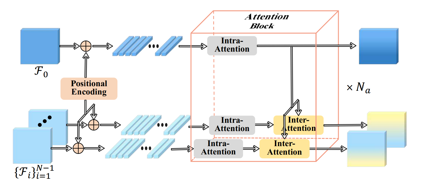
Fig 3. FMT block [1].
class EncoderLayer(nn.Module):
    def __init__(self, d_model, n_heads, d_keys=None, d_values=None, d_ff=None, dropout=0.0,
                 activation="relu"):
        super(EncoderLayer, self).__init__()
        d_keys = d_keys or (d_model//n_heads)
        inner_attention = LinearAttention()
        attention = AttentionLayer(inner_attention, d_model, n_heads, d_keys, d_values)

        d_ff = d_ff or 2 * d_model
        self.attention = attention
        self.linear1 = nn.Linear(d_model, d_ff)
        self.linear2 = nn.Linear(d_ff, d_model)
        self.norm1 = nn.LayerNorm(d_model)
        self.norm2 = nn.LayerNorm(d_model)
        self.dropout = nn.Dropout(dropout)
        self.activation = getattr(F, activation)
    def forward(self, x, source):
        # Normalize the masks
        N = x.shape[0]
        L = x.shape[1]
        # Run self attention and add it to the input
        x = x + self.dropout(self.attention(
            x, source, source,
        ))
        # Run the fully connected part of the layer
        y = x = self.norm1(x)
        y = self.dropout(self.activation(self.linear1(y)))
        y = self.dropout(self.linear2(y))
        return self.norm2(x+y)
With extracted features, TransMVSNet then reconstructs correlation volume. To obtain the reconstructed volume, the relationship between a pixel p in a reference feature and p hat at at the source feature view is defined by
\[\mathbf{\hat{p}} = \mathbf{K}[\mathbf{R}(\mathbf{K_0^{-1}} \mathbf{p} d) + \mathbf{t}]\]Where R is the rotation matrix and t is the translation matrix between the two views. \(K_0\) and \(K\) are intrinsic matrices of the reference and source camera. To make the resolution consistent, feature maps also undergo a binary interpolation. Thereby, we obtain the pairwise feature correlation at p:
\[c_i^{(d)}(p) = <\mathbf{F}_0(\mathbf{p}), \mathbf{\hat{F}}_i^{(d)}P(\mathbf{p})>\]where Fi is the i-th source feature map at depth p. From these pairwise correlations, we finally obtain the volume defined as
\[C^{(d)}(\mathbf{p}) = \sum_{i=1}^{N-1} \max_d \{c_i^{(d)}{\mathbf{p}} \cdot c_i^{(d)} (\mathbf{p}) \}\]The following code implements TransMVSNet 3D reconstruction from extracted features.
for i, (src_fea, src_proj) in enumerate(zip(src_features, src_projs)): # src_fea: [B, C, H, W]
    src_proj_new = src_proj[:, 0].clone() # [B, 4, 4]
    src_proj_new[:, :3, :4] = torch.matmul(src_proj[:, 1, :3, :3], src_proj[:, 0, :3, :4])
    ref_proj_new = ref_proj[:, 0].clone() # [B, 4, 4]
    ref_proj_new[:, :3, :4] = torch.matmul(ref_proj[:, 1, :3, :3], ref_proj[:, 0, :3, :4])
    warped_volume = homo_warping(src_fea, src_proj_new, ref_proj_new, depth_values)
    similarity = (warped_volume * ref_feature.unsqueeze(2)).mean(1, keepdim=True)

    if view_weights == None:
        view_weight = self.pixel_wise_net(similarity) # [B, 1, H, W]
        view_weight_list.append(view_weight)
    else:
        view_weight = view_weights[:, i:i+1]

    if self.training:
        similarity_sum = similarity_sum + similarity * view_weight.unsqueeze(1) # [B, 1, D, H, W]
        pixel_wise_weight_sum = pixel_wise_weight_sum + view_weight.unsqueeze(1) # [B, 1, 1, H, W]
    else:
        similarity_sum += similarity * view_weight.unsqueeze(1)
        pixel_wise_weight_sum += view_weight.unsqueeze(1)
After obtaining the reconstruction, TransMVSNet applies a focal loss function that treats this reconstruction task as a classification task. The focal loss at each depth estimation is given by
\[L = \sum_{\mathbf{p} \in \{\mathbf{p}_v\}} -(1-P^{(\tilde{d})}(\mathbf{p}))^\gamma \log \big ( P^{(\tilde{d})} (\mathbf{p})\big )\]where \(P^{(d)}(\mathbf{p})\) denotes the predicted probability of \(d\) as pixel \(\mathbf{p}\). \(\tilde{d}\) is the depth value that is closest to the ground truth. \(\{ \mathbf{p}_v \}\) represents a subset of pixels with valid ground truths. \(\gamma\) is the focusing parameter, and this loss becomes cross entropy loss with this value set to 0.
Results and Discussion
The performance of TransMVSNet is measured by the average of accuracy and completeness. Accuracy of MVS tasks measures the mean absolute point-cloud-to-point-cloud distance between the ground truth and the reconstruction. Completeness evaluates the percentage of the ground truth 3D points that are correctly reconstructed in the output model.
The first thing we would like to note is that TransMVSNet shows good generalizability and performs well both in indoor and outdoor data. The DTU dataset contains images of objects, whereas Tanks and Temples dataset contains indoor and outdoor scenes. In the paper, the authors have demonstrated that the use of Feature Matching Transformer (FMT) enhances TransMVSNet’s effectiveness in real-world scenes.
Secondly, we have also noticed a difference between our visualization of depth maps and those presented in the paper. Fig. 4 shows five examples of depth maps TransMVSNet generates in one case. One difference between our visualization the ones in the paper is that our depth maps include noise in the background. The objects in the depth maps contain a smooth surface, whereas the background shows more variation in depth values. However, the depth maps presented in the paper contains less noise in the background, as shown in Fig. 2. This is because depth filtering and fusion is applied to reduce noise in depth data. In TransMVSNet, this task is done with a dynamic checking strategy that involves both confidence thresholding and geometric consistency.
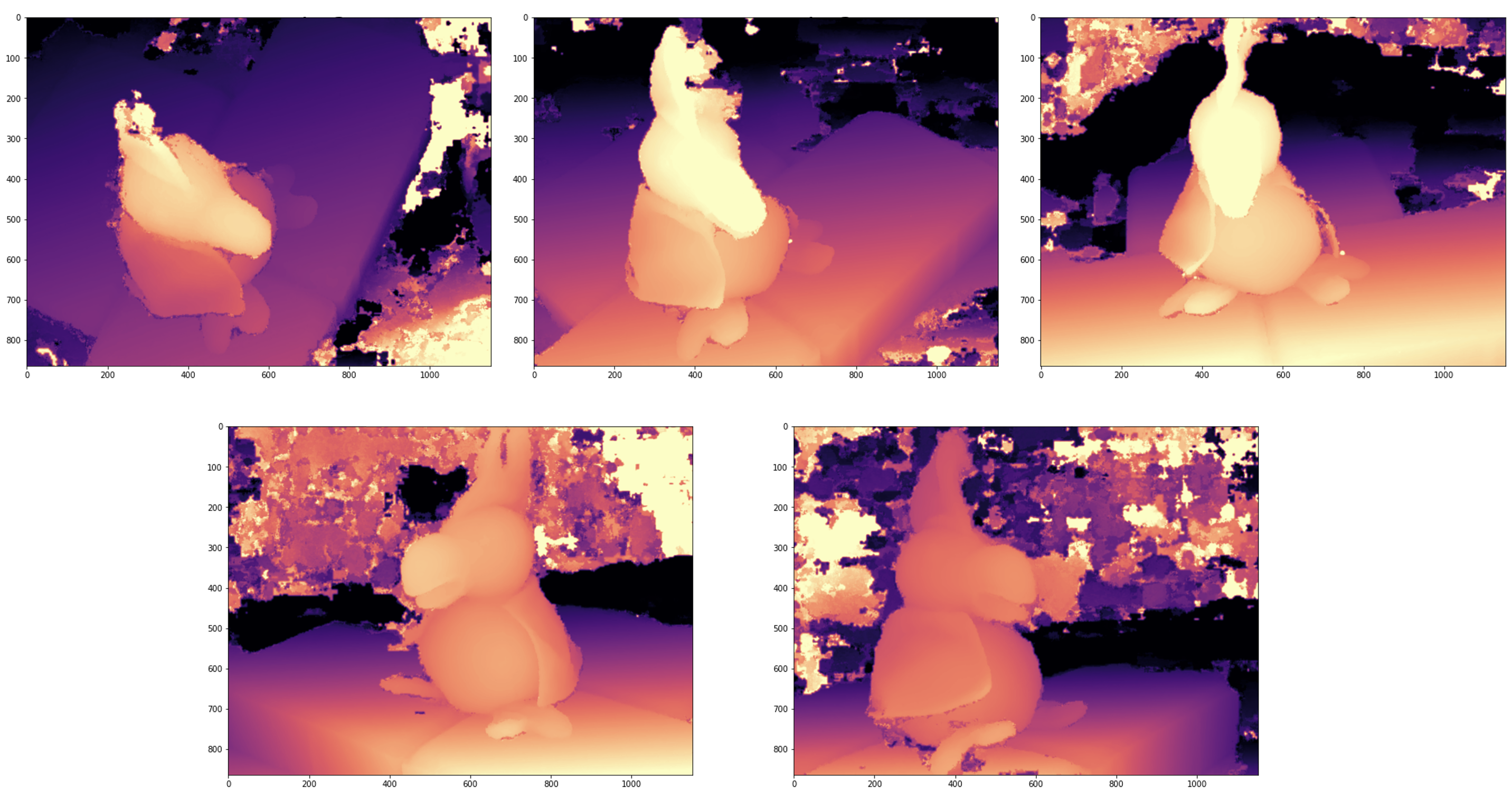
Fig 4. 5 depth maps from DTU test set.
Moreover, TransMVSNet, as one of the start-of-the-art MVS frameworks, reveals a general challenge in MVS task. Fig. 5 shows our visualization of 3D point cloud of case 4 in DTU testing set. From this example, we could see that the point cloud prediction is less dense in occluded regions such us the region between the feet of the toy duck and the underlying surface.
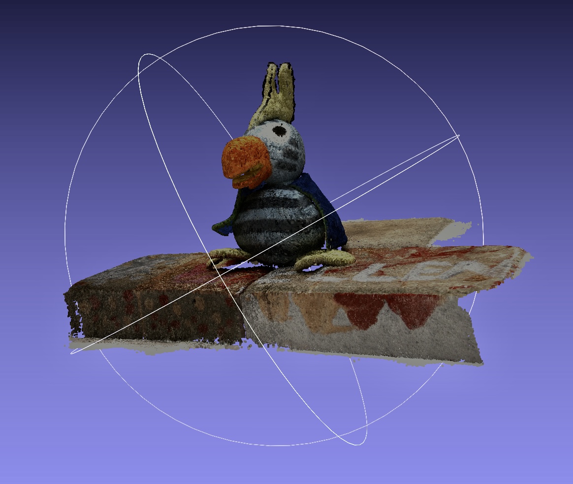
Fig 5. Visualization of point cloud.
Finally, TransMVSNet is a computationally expensive method, as it involves processing multiple input images and producing dense depth maps for each pixel with attention mechanism. This can be a bottleneck when processing large datasets or real-time applications. One way to improve the efficiency of the network is to reduce the resolution of the input images or the output depth maps, or to use a more lightweight network architecture.
CDS-MVSNet
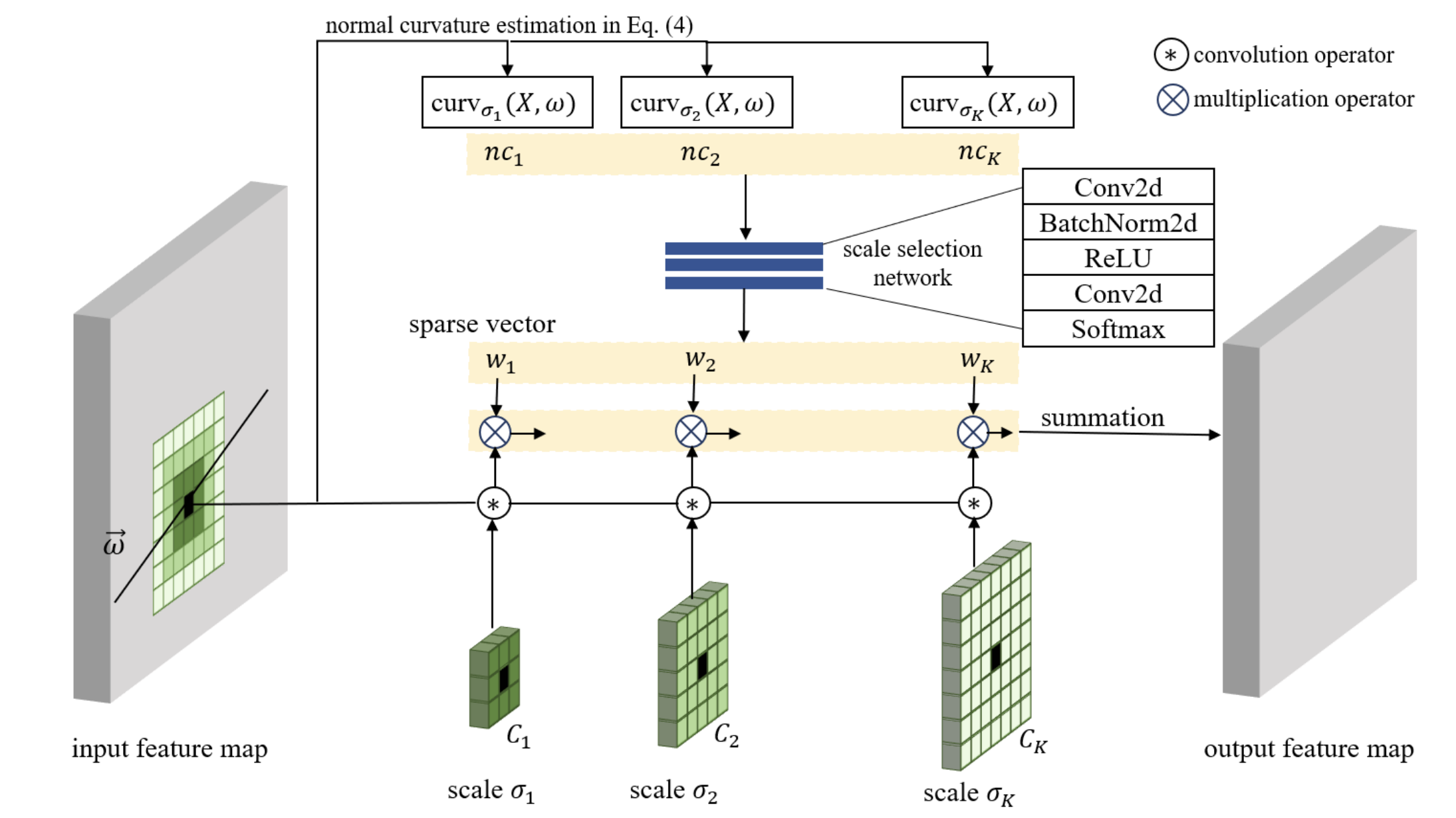
Fig 6. CDS-MVSnet architecture [3].
Motivation
Learning-based MVS methods are usually better than traditional methods at ambiguity and high computational complexity matching. The learning-based methods are usually composed of three steps: feature extraction, cost volume formulation, and cost volume regularization. Many researches have been conducted on the latter two steps, whereas the authors of CDS-MVSnet propose a novel feature extraction network, the CDSFNet. It is composed of multiple novel convolution layers, each of which can select a proper patch scale for each pixel guided by the normal curvature of the image surface.
Architecture and Code Implementation
Curvature-Guided Dynamic Scale Convolution(CDSConv)
The formula of normal curvature of a patch centered at \(X\) along the direction of epipolar line \(\omega=[u,v]^T\) can be written as follows
\[curv_\sigma(X,\omega)={u^2I_{xx}(X,\sigma)+2uvI_{xy}(X,\sigma)+v^2I_{yy}(X,\sigma) \over \sqrt{1+I_x^2(X,\sigma)+I_y^2(X,\sigma)}(1+(uI_x(X,\sigma)+vI_y(X,\sigma)))}\]where \(I(X,\sigma) = I(X)*G(X,\sigma)\) is the image intensity of pixel \(X\) in the image scale \(\sigma\); it is determined by convolving \(I\) with a Gaussian kernel \(G(X, \sigma)\) with the window size/scale \(\sigma\).
There are two main drawbacks when embedding the normal curvature into a deep neural network. First, the computation is heavy because of convolution operations for computing the derivatives of \(I\). Second, using the formula to compute curvature is infeasible when the pixel \(X\) is a latent feature \(F^{in}(X)\) instead of the image intensity \(I(X)\). For these reasons, the authors propose e learnable normal curvature having the formula as follows
\[curv_\sigma(X,\omega)=\omega \begin{bmatrix} F^{in}*K_\sigma^{xx} & F^{in}*K_\sigma^{xy} \\ F^{in}*K_\sigma^{xy} & F^{in}*K_\sigma^{yy} \end{bmatrix} \omega^T\]where \(K ^{(.)} _\sigma\) s are the learnable kernels and \(\|\|K ^{(.)} _\sigma \|\| \to 0\), \(F^{in}\) is the input feature.
After the normal curvatures are calculated in candidate scales \(\sigma\), proper scale is selected for each pixel through a lightweight CNN with two convolutional blocks. The output feature has formula as follows:
\[F^{out}=w_1(F^{in}*C_1)+w_2(F^{in}*C_2)+\cdots+w_K(F^{in}*C_K)\]where \(∗\) is the convolution operator. Also, the normal curvature corresponding to the selected scale is extracted by
\[NC^{est}=w_1curv_{\sigma_1} + w_2curv_{\sigma_2} +\cdots+w_Kcurv_{\sigma_K}\]The code for the CDSConv is implemented as follows
class  DynamicConv(nn.Module):

	def  __init__(self, in_c, out_c, size_kernels=(3, 5, 7), stride=1, bias=True, thresh_scale=0.01, **kwargs):
		super(DynamicConv, self).__init__()
		self.size_kernels = size_kernels
		self.thresh_scale = thresh_scale
		self.att_convs = nn.ModuleList([nn.Conv2d(in_c, 3, k, padding=(k-1)//2, bias=False) for  k  in  size_kernels])
		self.convs = nn.ModuleList([nn.Conv2d(in_c, out_c, k, padding=(k-1)//2, stride=stride, bias=bias) for  k  in  self.size_kernels])
		hidden_dim = kwargs.get("hidden_dim", 4)
		self.att_weights = nn.Sequential(nn.Conv2d(len(size_kernels), hidden_dim, 1, bias=False),
		nn.BatchNorm2d(hidden_dim),
		nn.ReLU(inplace=True),
		nn.Conv2d(hidden_dim, len(size_kernels), 1, bias=False))

		for  p  in  self.att_convs.parameters():
			torch.nn.init.normal_(p, std=0.1)

	def  forward(self, feature_vol, epipole=None, temperature=0.001):
		# surface = feature_vol.mean(dim=1, keepdim=True)
		batch_size, height, width = feature_vol.shape[0], feature_vol.shape[2], feature_vol.shape[3]
		y, x = torch.meshgrid([torch.arange(0, height, dtype=torch.float32, device=feature_vol.device),
		torch.arange(0, width, dtype=torch.float32, device=feature_vol.device)])
		x, y = x.contiguous(), y.contiguous()
		epipole_map = epipole.unsqueeze(-1).unsqueeze(-1) # [B, 2, 1, 1]
		u = x.unsqueeze(0).unsqueeze(0) - epipole_map[:, [0], :, :] # [B, 1, H, W]
		v = y.unsqueeze(0).unsqueeze(0) - epipole_map[:, [1], :, :] # [B, 1, H, W]
		normed_uv = torch.sqrt(u**2 + v**2)
		u, v = u / (normed_uv + 1e-6), v / (normed_uv + 1e-6)

		curvs = []
		results = []

		for  idx, s  in  enumerate(self.size_kernels):
			curv = self.att_convs[idx](feature_vol)
			curv = (curv * torch.cat((u**2, 2*u*v, v**2), dim=1)).sum(dim=1, keepdim=True)
			# w = self.att_weights[idx](feature_vol)
			curvs.append(curv) #.unsqueeze(1))
			results.append(self.convs[idx](feature_vol).unsqueeze(1))

		curvs = torch.cat(curvs, dim=1) # [B, num_kernels, H, W]
		weights = self.att_weights(curvs)
		weights = F.softmax(weights / temperature, dim=1)
		filtered_result = (torch.cat(results, dim=1) * weights.unsqueeze(2)).sum(dim=1)
		norm_curv = (curvs * weights).sum(dim=1, keepdim=True)
		return  filtered_result, norm_curv  #, sum_mask, t11, t12, t13
Curvature-Guided Dynamic Scale Feature Network(CDSFNet)
The CDSFNet, used as the feature extraction step for the CDS-MVS framework, can select the optimal scale for each pixel to learn robust representation that reduces matching ambiguity. Given the inputs including image \(I\) and its estimated epipole \(e\), the network outputs three features for three level of spatial resolution \(\{F^{(0)},F^{(1)},F^{(2)}\}\) and three estimated normal curvatures \(\{NC^{est,(0)},NC^{est,(1)},NC^{est,(2)}\}\).
The code for CDSFNet is implemented as follows:
class  FeatureNet(nn.Module):

def  __init__(self, base_channels, num_stage=3, stride=4, arch_mode="unet"):

	super(FeatureNet, self).__init__()
	assert  arch_mode  in ["unet", "fpn"], print("mode must be in 'unet' or 'fpn', but get:{}".format(arch_mode))
	print("*************feature extraction arch mode:{}****************".format(arch_mode))
	self.arch_mode = arch_mode
	self.stride = stride
	self.base_channels = base_channels
	self.num_stage = num_stage
	self.conv00 = Conv2d(3, base_channels, (3, 7, 11), 1, dynamic=True)
	self.conv01 = Conv2d(base_channels, base_channels, (3, 5, 7), 1, dynamic=True)
	self.downsample1 = Conv2d(base_channels, base_channels*2, 3, stride=2, padding=1)
	self.conv10 = Conv2d(base_channels*2, base_channels*2, (3, 5), 1, dynamic=True)
	self.conv11 = Conv2d(base_channels*2, base_channels*2, (3, 5), 1, dynamic=True)
	self.downsample2 = Conv2d(base_channels*2, base_channels*4, 3, stride=2, padding=1)
	self.conv20 = Conv2d(base_channels*4, base_channels*4, (1, 3), 1, dynamic=True)
	self.conv21 = Conv2d(base_channels*4, base_channels*4, (1, 3), 1, dynamic=True)
	self.out1 = DynamicConv(base_channels*4, base_channels*4, size_kernels=(1, 3))
	self.act1 = nn.Sequential(nn.InstanceNorm2d(base_channels*4), nn.Tanh())
	self.out_channels = [base_channels*4]
	self.inner1 = Conv2d(base_channels * 6, base_channels * 2, 1)
	self.inner2 = Conv2d(base_channels * 3, base_channels, 1)
	self.out2 = DynamicConv(base_channels*2, base_channels*2, size_kernels=(1, 3))
	self.act2 = nn.Sequential(nn.InstanceNorm2d(base_channels*2), nn.Tanh())
	self.out3 = DynamicConv(base_channels, base_channels, size_kernels=(1, 3))
	self.act3 = nn.Sequential(nn.InstanceNorm2d(base_channels), nn.Tanh())
	self.out_channels.append(base_channels*2)
	self.out_channels.append(base_channels)


def  forward(self, x, epipole=None, temperature=0.001):

	conv00, nc00 = self.conv00(x, epipole, temperature)
	conv01, nc01 = self.conv01(conv00, epipole, temperature)
	down_conv0, down_epipole0 = self.downsample1(conv01), epipole / 2
	conv10, nc10 = self.conv10(down_conv0, down_epipole0, temperature)
	conv11, nc11 = self.conv11(conv10, down_epipole0, temperature)
	down_conv1, down_epipole1 = self.downsample2(conv11), epipole / 4
	conv20, nc20 = self.conv20(down_conv1, down_epipole1, temperature)
	conv21, nc21 = self.conv21(conv20, down_epipole1, temperature)
	intra_feat = conv21
	outputs = {}
	out, nc22 = self.out1(intra_feat, epipole=down_epipole1, temperature=temperature)
	out = self.act1(out)
	nc_sum = (nc20 ** 2 + nc21**2 + nc22 ** 2) / 3
	outputs["stage1"] = out, nc_sum, nc22.abs()
	intra_feat = torch.cat((F.interpolate(intra_feat, scale_factor=2, mode="nearest"), conv11), dim=1)
	intra_feat = self.inner1(intra_feat)
	out, nc12 = self.out2(intra_feat, epipole=down_epipole0, temperature=temperature)
	out = self.act2(out)
	nc_sum = (nc10 ** 2 + nc11 ** 2 + nc12 ** 2) / 3
	outputs["stage2"] = out, nc_sum, nc12.abs()
	intra_feat = torch.cat((F.interpolate(out, scale_factor=2, mode="nearest"), conv01), dim=1)
	intra_feat = self.inner2(intra_feat)
	out, nc02 = self.out3(intra_feat, epipole=epipole, temperature=temperature)
	out = self.act3(out)
	nc_sum = (nc00 ** 2 + nc01 ** 2 + nc02 ** 2) / 3
	outputs["stage3"] = out, nc_sum, nc02.abs()
	return  outputs
CDS-MVSNet
The CDS-MVSNet adopted the cascade structure of CasMVSNet [5] as the baseline structure. The network is composed of multiple cascade stages to predict the depth maps in a coarse-to-fine manner. Each stage estimates a depth through three steps: feature extraction, cost volume formulation, cost volume regularization & depth regression. CDS-MVSNet formulates a 3D cost volume based on the output features of CDSFNet. The features of CDSFNet effectively reduce the matching ambiguity by considering the proper pixel scales.
Discussion
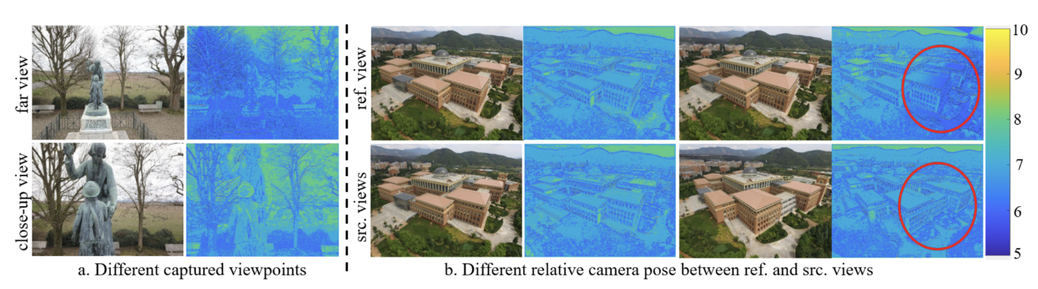
Fig 7. scale map of CDS-MVSNet [3].
The CDS-MVSNet is good at extracting features of images with different viewpoints and camera pose. In Fig. 7a, the closer viewpoint is, the larger scales are estimated on the scale map. In Fig. 7b, the reference and source scale maps are similar when the difference of camera poses is small. And when it is large, the scale map of reference view is changed to adapt the source view, which is marked in the red circle.
Also, with the stacking of mutiple CDSConvlayers layers, the searching scale-space is expanded profoundly even when only 2-3 candidate kernel scales are chosen at each layer. This helps in reducing the complexity of the model significantly.
Comparing TransMVSNet and CDS-MVSNet
As shown in figure 8, CDS-MVSNet predictions are clearer on the edges of objects and have fewer noises in the backgroud.
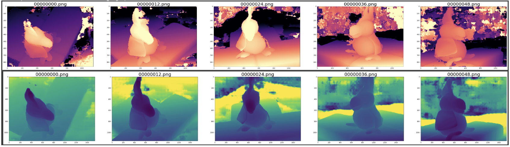
Fig 8. Depth map of CDS-MVSNet Output [3].
As shown in table 1, when having similar results on the DTU test dataset, CDS-MVSNet has a slightly less complex model and a much faster prediction speed per image than the TransMVSNet.
| model | learnable params | average prediction time/image (sec) | Acc. | Comp. | Overall |
|---|---|---|---|---|---|
| TransMVSNet | 1148924 | 2.13 | 0.321 | 0.289 | 0.305 |
| CDS-MVSNet | 981622 | 1.08 | 0.352 | 0.280 | 0.316 |
Table 1. Comparison Between two models(Acc., Comp., and Overall are DTU testing results, the lower the better)
Appendix
Code Base: https://colab.research.google.com/drive/1vdBaPXzHRh5jkdQUMWRb9Jy-cnMCCtdL?usp=sharing.
Spotlight Video: https://www.youtube.com/watch?v=Mu6Q2pgj66Q.
Reference
[1] Aanæs, H., Jensen, R.R., Vogiatzis, G. et al. Large-Scale Data for Multiple-View Stereopsis. Int J Comput Vis 120, 153–168 (2016).
[2] Ding, Yikang, et al. “Transmvsnet: Global context-aware multi-view stereo network with transformers.” Proceedings of the IEEE/CVF Conference on Computer Vision and Pattern Recognition. 2022.
[3] Giang, Khang Truong, Soohwan Song, and Sungho Jo. “Curvature-guided dynamic scale networks for multi-view stereo.” arXiv preprint arXiv:2112.05999 (2021).
[4] Tsung-Yi Lin, Piotr Dollar, Ross Girshick, Kaiming He, Bharath Hariharan, and Serge Belongie. Feature pyramid networks for object detection. In Proceedings of the IEEE conference on computer vision and pattern recognition, pages 2117–2125, 2017.
[5] Xiaodong Gu, Zhiwen Fan, Siyu Zhu, Zuozhuo Dai, Feitong Tan, and Ping Tan. Cascade cost volume for high-resolution multi-view stereo and stereo matching. In Proceedings of the IEEE/CVF Conference on Computer Vision and Pattern Recognition, pp. 2495–2504, 2020.