Investigation on the Robustness of CLIP
Topic: CLIP: Text-image joint embedding
- Demo Video
- Abstract
- Introduction
- Experiment Design
- Technical Details
- Experiment Result
- Discussion
- Reference
Demo Video
Abstract
This project investigates the robustness of the CLIP model by experimenting with image retrieval using clip-retrieval. We used 2 datasets and 3 data augmentation/manipulation techniques to generate a variety of image embedding, and query a list of similar embedding with clip-retieval through “query by embedding”. We then calculate the similarity and accuracy of such retrieval by calculating and analyzing the distance between the query and retrieved image embedding with a pre-set threshold. After retrieving and analyzing over 5k original images and 50k search result, we observes that the CLIP model exhibits strong robustness across different types of images. However, it is less robust to “cropping” manipulations on images with strong facial features, and less robust to “blurred” and “grey” manipulation on scene images.
Introduction
CLIP is a neural network created by open.ai that can effectively learn visual concepts from natural language supervision. CLIP shows compelling performance in zero-shot image classification. Our motivation is to examine the robustness of the CLIP model against data poisoning attacks. We plan to conduct multiple experiments with various datasets and data-poisoning techniques and get insights into the accuracy and performance of CLIP model on image classification and image retrieval.
What is CLIP
CLIP (Contrastive Language-Image Pre-Training) is a neural network created by open.ai that can effectively learn visual concepts from natural language supervision. CLIP is capable of performing various tasks such as image and text classification, zero-shot learning, and image captioning. It works by using a contrastive learning approach to learn a joint embedding space for images and text, where similar images and text are placed close together while dissimilar ones are separated. CLIP’s ability to relate images and text without explicit training on specific tasks has made it a powerful tool for a wide range of applications, including natural language processing, computer vision, and robotics.
The CLIP model is implemented as a neural network that consists of a vision transformer and a language transformer. During pre-training, the model learns to predict which text caption corresponds to a given image and which image corresponds to a given text caption. The CLIP model architecture also includes several technical innovations, such as multi-modal input tokenization and a normalization technique called adaptive gradient clipping. Once pre-trained, the CLIP model can be fine-tuned on various downstream tasks, such as image classification, natural language processing, and image retrieval, by adjusting the weights of the neural network to fit the specific task at hand. The performance of the CLIP model has been shown to exceed the state-of-the-art on several benchmark datasets.
What is clip-retrieval
clip-retrieval is implemented by using the CLIP model to create embeddings of natural language queries and images. Given a query, the clip-retrieval model computes an embedding of the query and compares it to the embeddings of a database of images using a similarity measure. The model then retrieves the images that are most similar to the query based on their embedding similarity score. The model can be fine-tuned on specific retrieval tasks by adjusting the similarity measure or incorporating additional information during training.
“Query by embedding” is a search technique that involves comparing the embeddings of a query (e.g., an image or a text) with the embeddings of a database of items to find the most similar items. clip-retrieval is a specific implementation of query by embedding that uses the CLIP model to create embeddings of images and natural language queries. By comparing the embeddings of a query with the embeddings of a database of images, clip-retrieval can retrieve the most relevant images that match the query. This approach allows for more flexible and natural search queries, as users can express their search intent in natural language without needing to provide specific keywords or image features.
Project Goal
This project investigates the robustness of the CLIP model by experimenting with image retrieval using clip-retrieval.
We plan on using the clip model to generate a embedding for each query image, and retrieve a list of image with clip-retrieval using the embedding. We plan on comparing query image and retrieved image by calculating the distance/similarity between the embeddings. Furthermore, We plan on using two dataset and three image manipulation techniques. we plan on manipulating the query images with 3 different image manipulation techniques (cropped, blurred, grey). We plan on comparing the retrieving robustness of the CLIP model among these manipulation techniques. At the same time, we plan on experiments with two different dataset, NBA players and Miniplaces. The NBA player dataset contains images with player’s facial features, while Miniplaces does not. By the conclusion of the experiment, we hope to get insights on the robustness of the image retrieval ability of CLIP.
Experiment Design
To test the robustness of the model, we employed two distinct datasets: one pertaining to NBA players from the years 2021-2022, featuring images of the players in various poses, and another called MiniPlace that comprises scenes from both indoor and outdoor environments. We intend to use these two distinct dataset to see the different performance and robustness of the model to figure images and scene images.
For the NBA player dataset, there are images for 490 players and about 60 images for each player. Due to the time constraint and the limitation of GPU resources. We randomly select 70 players in the dataset for our experiment and let S denote the partial set.
For each player P in S, we pick one of his images \(x_i^P\) as the query image and transform it to its vector representation/embedding. \(v_i^P = f(x_i^P)\), where \(f\) is the transformation function. We then pass the query-image embedding to the CLIP-Retrieval to get a list of query results.
After we get the query result, we calculate the L2 distance between the query result and the original image for each query result in the result list. Next, we compare the distance for each query result with a pre-set threshold: t = 0.8; if the distance is greater than t, we will count it as an inaccurate result since a greater distance between the query results represents a large dissimilarity between two images.
Finally, we calculate the accuracy of the model using \(v_i^P\) as the query image by using the formula: \(\frac{\text{numbers of query result that has a l2 distance less than 0.8}}{\text{total number of query result}}\). Therefore, for each player, we will have N accuracy where N equals the number of images of that player.
Thus, we can calculate the accuracy for each player by taking the average of the N result. Also, by taking the average of all the accuracy in the partial player dataset S, we can find the final accuracy for the model using the NBA player dataset.
Moreover, for each time we transform the image to image embedding, we can add one of the three image augmentation skills(blurring, randomly cropping, grey) in order to test the robustness of the model to data augmentation. Therefore, we will have four accuracy including the original image in total.
For the Miniplace dataset, we apply the same procedure here. We simply just replace “each player” in the NBA dataset with the “scene name” in the miniplace dataset.
Technical Details
Setup
Install clip-retrieval and Kaggle
!pip install clip-retrieval
!pip install -q kaggle
Install clip-retrieval client
from IPython.display import Image, display
from clip_retrieval.clip_client import ClipClient, Modality

IMAGE_BASE_URL = "https://github.com/rom1504/clip-retrieval/raw/main/tests/test_clip_inference/test_images/"

def log_result(result):
    id, caption, url, similarity = result["id"], result["caption"], result["url"], result["similarity"]
    print(f"id: {id}")
    print(f"caption: {caption}")
    print(f"url: {url}")
    print(f"similarity: {similarity}")
    display(Image(url=url, unconfined=True))

client = ClipClient(
    url="https://knn.laion.ai/knn-service",
    indice_name="laion5B-L-14",
    aesthetic_score=9,
    aesthetic_weight=0.5,
    modality=Modality.IMAGE,
    num_images=10,
)
Load CLIP model
model, preprocess = clip.load('ViT-L/14', device=device)
Dataset
We used two different datasets: NBA Player Image Dataset 2019-20 from Kaggle, and the Miniplaces dataset from Assignment 1
NBA players
!kaggle datasets download -d djjerrish/nba-player-image-dataset-201920
!unzip nba-player-image-dataset-201920.zip
Minipalces
!pip3 install --upgrade gdown --quiet
!gdown 1CyIQOJienhNITwGcQ9h-nv8z6GOjV2HX
tar = tarfile.open("data.tar.gz", "r:gz")
# Extract the file to the "/Miniplaces" folder
total_size = sum(f.size for f in tar.getmembers())
with tqdm(total=total_size, unit="B", unit_scale=True, desc="Extracting tar.gz file") as pbar:
    for member in tar.getmembers():
        tar.extract(member, os.path.join(root_dir))
        pbar.update(member.size)
tar.close()
Generate Image Embedding
def get_image_emb(image_path):
    with torch.no_grad():
        image = pimage.open(image_path)
        image_emb = model.encode_image(preprocess(image).unsqueeze(0).to("cuda"))
        image_emb /= image_emb.norm(dim=-1, keepdim=True)
        image_emb = image_emb.cpu().detach().numpy().astype("float32")[0]
        return image_emb
Manipulation techniques
Blurred
def get_blurred_emb(image_path):
    with torch.no_grad():
        image_np = cv2.imread(image_path)   # reads an image in the BGR format
        image_np = cv2.cvtColor(image_np, cv2.COLOR_BGR2RGB)
        # Split RGB channels
        r, g, b = image_np[:,:,0], image_np[:,:,1], image_np[:,:,2]
        # Apply Gaussian filter to each channel
        r_blurred = ndimage.gaussian_filter(r, sigma=3)
        g_blurred = ndimage.gaussian_filter(g, sigma=3)
        b_blurred = ndimage.gaussian_filter(b, sigma=3)
        # Merge blurred channels
        blurred_image = np.stack([r_blurred, g_blurred, b_blurred], axis=2)
        blurred_image = pimage.fromarray(np.uint8(blurred_image))
        image = blurred_image
        image_emb = model.encode_image(preprocess(image).unsqueeze(0).to("cuda"))
        image_emb /= image_emb.norm(dim=-1, keepdim=True)
        image_emb = image_emb.cpu().detach().numpy().astype("float32")[0]
        return image_emb
Cropped
def get_cropping_emb(image_path):
    with torch.no_grad():
        image_pil = pimage.open(image_path)
        # Generate random crop dimensions
        width, height = image_pil.size
        crop_size = min(width, height) # Maximum crop size
        left = random.randint(0, width - crop_size)
        top = random.randint(0, height - crop_size)
        right = left + crop_size
        bottom = top + crop_size
        # Crop image
        cropped_pil = image_pil.crop((left, top, right, bottom))
        image = cropped_pil
        image_emb = model.encode_image(preprocess(image).unsqueeze(0).to("cuda"))
        image_emb /= image_emb.norm(dim=-1, keepdim=True)
        image_emb = image_emb.cpu().detach().numpy().astype("float32")[0]
        return image_emb
Grey
def get_grey_emb(image_path):
    with torch.no_grad():
        image_pil = pimage.open(image_path)
        image_pil = pimage.open(image_path).convert('L')
        image = image_pil
        image_emb = model.encode_image(preprocess(image).unsqueeze(0).to("cuda"))
        image_emb /= image_emb.norm(dim=-1, keepdim=True)
        image_emb = image_emb.cpu().detach().numpy().astype("float32")[0]
        return image_emb
Calculate Accuracy
import os
from tqdm.notebook import tqdm
import torch
import random
import json
def find_accuracy(rootdir, player_names, start, step, manipulation = None, mani_name="original"):
    player_rootdir = rootdir
    total_player = len(player_names)
    player_names = player_names[start:min(total_player, start+step)]
    print("current batch players:\n", player_names)
    accuracy_for_players = {}
    total_acc = []# total_acc is for the calculation for the global accuracy
    for player in tqdm(player_names): # Generate embedding for each image for this one player
      img_emb = []
      poison_emb = []
      accuracy_for_players[player] = []
      image_path = os.path.join(player_rootdir, player, player_img)
      for player_img in os.listdir(os.path.join(player_rootdir, player)):
        img_emb.append(get_image_emb(image_path))
      # Now, set one embedding as the query image and calculate the accuracy for this image
        if manipulation is not None:
          poison_emb.append(manipulation(image_path))
      ## acc_list is used to store the accuracies using different embedding of the same players
      acc_list = []

      threshold = 0.80
      print("\nthreshold = ", t)
      for i in tqdm(range(len(img_emb)),desc=player+" inside progress:", position=0, leave=True):
        embedding = poison_emb[i] if manipulation is not None else img_emb[i]
        search_result = client.query(embedding_input = embedding.tolist())
        length = len(search_result)
        success_length = 0
        if length == 0: # skip if there is no search result available
          continue
        valid_search_results = []
        for result in search_result:
          url = result['url']
          succeed, result_emb = get_image_url_emb(url)
          if succeed:
            success_length += 1
            distance = torch.dist(torch.from_numpy(result_emb),torch.from_numpy(img_emb[i]))
            if distance < threshold:
              valid_search_results.append(result)
        if success_length == 0: # again, skip if there is no search result available
          continue
        acc = len(valid_search_results)/success_length
        acc_list.append(acc)
      accuracy_for_players[player] = acc_list
      if len(acc_list) == 0:
        total_acc.append(0)
      else:
        print(player+"'s accuracy is ", sum(acc_list)/len(acc_list))
        total_acc.append(sum(acc_list)/len(acc_list))

      ############# Log data to json #####################
      with open('clip_output_'+mani_name+'.json', "w") as f:
          data[mani_name][player] = acc_list
          json.dump(data, f)
      ############# Log data to json #####################

    total_acc = sum(total_acc)/len(total_acc)
    return total_acc
Calculate Total Accuracy (among each category)
import statistics
import json
def calculate_total_miniplaces(output_file_path, mani_name):
  with open(output_file_path, "r") as f:
      data = json.load(f)
      total = []
      for key in data[mani_name]:
          if key != 'total':
            acc_list = data[mani_name][key]
            mean = statistics.mean(acc_list)
            total.append(mean)
  with open(output_file_path, "w") as f:
      data[mani_name]["total"] = total
      json.dump(data, f)

mani_names = ["original", "blurred", "cropped", "grey"]
for mani_name in mani_names:
  calculate_total_miniplaces('clip_output_miniplaces_'+mani_name+'.json', mani_name)
Experiment Result
** Calculated the average of the total accuracy for each combination of the dataset and manupulation techniques
| | Original | Blurred | Cropped | Grey |
|-------------|----------|---------|---------|--------|
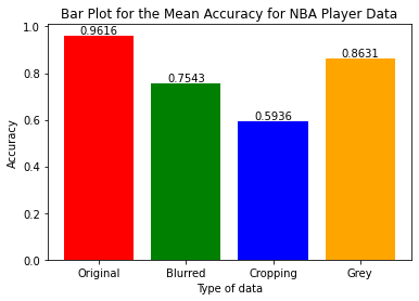
| NBA Players | 0.9615 | 0.7543 | 0.5936 | 0.8631 |
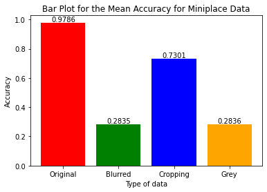
| MiniPlaces | 0.9786 | 0.2835 | 0.7301 | 0.2836 |
Output the experiment result into a JSON file
clip_output_NBA_original.json (shortened example)
{"original": {
  "Bacon, Dwayne": [1.0, 1.0, 1.0, 1.0, 1.0, 1.0, 1.0, 1.0, 0.8571428571428571, 1.0,1.0, 1.0, 1.0, 1.0, 1.0, 1.0, 1.0],
  "total": [0.9855334538878843, 1.0, 0.9849254159495123, 0.957936507936508, 0.9535211267605633, 1.0, 0.9366471734892787, 0.9808604336043361, 0.9692028985507246, 0.9547956771361027, 0.98642032570604, 0.9450743260267069, 0.9844377510040161, 0.9955197132616488, 0.949615975422427, 0.885477158343012, 0.9242630385487528, 0.9744331065759637, 0.9151648351648352, 0.9559374064091045, 0.9846153846153847, 0.9385353535353536, 0.9844806763285024, 0.977639751552795, 0.9753755668934241, 0.9367977528089888, 0.9361772486772487, 0.9914285714285714, 0.9122971285892634, 0.9805984555984556, 0.9644607843137255, 0.9613878446115288, 0.932716049382716, 1.0, 0.964010989010989, 0.9503164556962025, 0.9427628968253968, 0.9213675213675213, 0.9432252820807038, 0.9464285714285714, 0.9923469387755102, 0.9719211822660099, 0.9515160765160765, 0.9894179894179894, 0.9642512077294686, 0.933764367816092, 0.976010101010101, 0.9670454545454545, 0.9813034188034188, 0.9733606557377049, 0.9513513513513514],
  "Adams, Steven": [1.0, 1.0, 1.0, 1.0, 1.0, 1.0, 1.0, 1.0, 1.0, 1.0, 1.0, 1.0, 1.0, 1.0, 1.0, 1.0, 1.0]
  // More Players
  }}
clip_output_Miniplaces_Cropped.json (shortened example)
{"cropped": {
  "total": [0.15000000000000002, 0.6148922902494331, 0.5959807256235827, 0.7594160997732426, 0.8166553287981859, 0.7080839002267574, 0.723596733379342, 0.4625566893424036, 0.7150963718820862, 0.6887244897959184, 0.6202956061651714, 0.7148661454631604, 0.8752834467120182, 0.9306443970623075, 0.698109243697479, 0.9129251700680272, 0.8440842490842491, 0.540665719023928, 0.8138718820861678, 0.7356395215090867, 0.8890347805788982, 0.7968599033816425, 0.7906124141198768, 0.7365654474350126, 0.7953401360544218, 0.8714229024943311, 0.8315646258503402, 0.8106972789115646],
  "amusement_park": [0.0, 0.5, 0.0, 0.8333333333333334, 0.875],
  "art_gallery": [0.8571428571428571, 1.0, 0.75, 1.0, 0.4, 0.75, 0.3333333333333333, ],
  "aquarium": [1.0, 0.7142857142857143, 0.2222222222222222, 0.0, 0.0, 1.0, 1.0, 1.0, 1.0, 1.0, 1.0, 0.6666666666666666, 0.0, ],
  "aqueduct": [0.8571428571428571, 1.0, 0.875, 1.0, 0.0, 1.0, 0.8571428571428571, 0.8571428571428571]
  // More places
  }}
Discussion
After collecting the data and calculating the accuracy, we used numpy and matplotlib to visualize the data.
NBA Players Dataset Stats
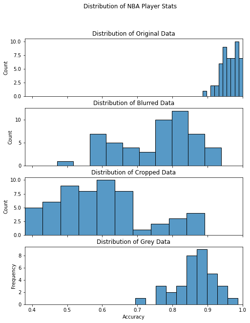
From the histogram we can see that the distribution of the four different data are all roughly normally distributed. Since there is a clearly difference between the mean value; therefore, we will use box plot to do further analysis.
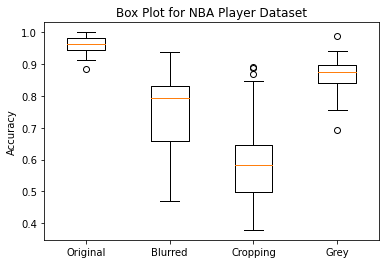
The box plot shows that the original dataset (no image manipulation) has the highest mean and lowest variance among the four datasets. Among the three datasets obtained by applying different data augmentation techniques, the cropping dataset has the lowest accuracy, while the grey dataset has a lower variance compared to the other two datasets.
Miniplaces Players Dataset Stats
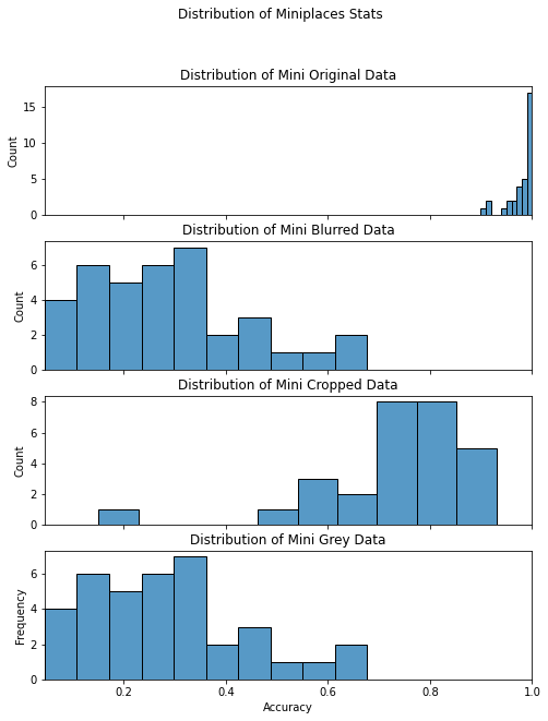
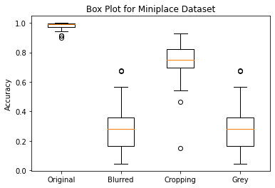
The result from the original dataset achieves the highest mean and lowest variance. Among the three query results using different data arugmentation techniques, cropped images has the highest mean value. It is also worth mentioning that the query results using different data arugmentation techniques have similar variance.
Comparison
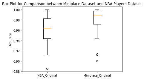
Since we want to compare the performance of the CLIP model with respect to different types of dataset, we will only use the original image data as comparison. From the box plot we can tell that the mean accuracy is roughly the same for the query result for NBA player and Miniplace; however, they have a slightly difference in variance.
Data Augmentaion vs Non Augmentation
For NBA Player data, the query results obtained through the use of the cropping technique have the lowest accuracy. It is plausible to suggest that when an image is randomly cropped, there is a high probability that the cropped portion may include part of or all of the facial features of a person, which will significantly affect the accuracy of the result.
Additionally, the lower variance in the results obtained from the greying technique could be attributed to the fact that converting the image to grey scale does not significantly alter the underlying information in the image data.
It is reasonable to conclude that in the Miniplace dataset, random cropping of a portion of the original image does not significantly affect the overall information of the data. However, blurring and converting the image to grayscale result in global effects, such as color elimination, which can lead to information loss in the original data, leading to lower accuracy scores.
Figure Image vs Scene Image
Upon comparing the image data of NBA players and Miniplace scenes, we can observe that although there is a slight difference in accuracy between the two datasets, it is not statistically significant. This indicates that there is no discernible difference in performance when using figure data versus scene data in the CLIP model. Furthermore, any minor differences in variance may be attributed to the differences in the selection of datasets, rather than the performance of the CLIP model.
Summary
To summarize, the CLIP model exhibits strong robustness across different types of images. However, it is less robust to “cropping” manipulations on figure data, as the centralized concentration of image information in figure images makes them more vulnerable to such manipulations. Additionally, the model is less robust to “blurred” and “grey” augmentations on scene data, as the dispersed concentration of image information in scene data makes them more susceptible to information loss through such manipulations.
Reference
Learning Transferable Visual Models From Natural Language Supervision
http://proceedings.mlr.press/v139/radford21a/radford21a.pdf
Language Models are Few-Shot Learners
https://papers.nips.cc/paper/2020/file/1457c0d6bfcb4967418bfb8ac142f64a-Paper.pdf
Self-training with Noisy Student improves ImageNet classification
https://openaccess.thecvf.com/content_CVPR_2020/papers/Xie_Self-Training_With_Noisy_Student_Improves_ImageNet_Classification_CVPR_2020_paper.pdf [1] Redmon, Joseph, et al. “You only look once: Unified, real-time object detection.” Proceedings of the IEEE conference on computer vision and pattern recognition. 2016.
Face Recognition in the age of CLIP & Billion image datasets
[https://arxiv.org/pdf/2301.07315.pdf] Bhat, A., & Jain, S. (2023, January 18). Face recognition in the age of clip & billion image datasets. arXiv.org. Retrieved March 26, 2023, from https://arxiv.org/abs/2301.07315