Deepfake Generation
This blog details Shrea Chari and Dhakshin Suriakannu’s project for the course CS 188: Computer Vision. This project discusses the topic of Deepfake Generation and takes a deep dive into three of the most popular models: Cycle-GAN, StarGAN and StyleGAN.
- Overview
- What Are “Deep Fakes”?
- Generative Adversarial Networks
- Image to Image Translation
- Unpaired Image to Image Translation
- Most popular GANs
- Cycle-GAN Networks
- StarGAN
- StarGAN v2
- StyleGAN
- StyleGAN v3
- Comparisons and Conclusions
- Demo Links
- References
Overview
What Are “Deep Fakes”?
“Deep Fakes” are synthetic media created using artificial intelligence. In current times, Deep Fake technology has been used to generate “fake” images or videos meant to look like they were captured in the real world.
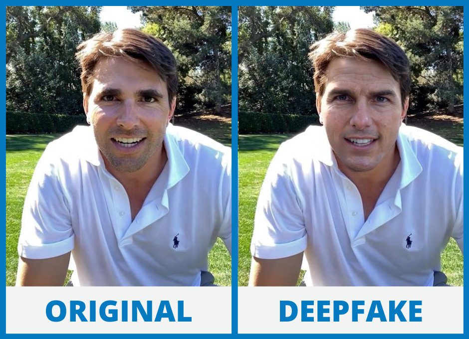
Deep Fake made of actor Tom Cruise. (Image source: https://www.trymaverick.com/blog-posts/are-deep-fakes-all-evil-when-can-they-be-used-for-good)
A popular subset of Deep Fakes can be found in face swapped images and videos, as shown above. This blog will detail various approaches to Deep Fake generation and analyze their strengths and weaknesses.
With the ease of access to tools such as AI and the lack of paired training data needed to generate this content, the deceptive prowess of Deep Fakes has become concerning to many around the world. As a result, Deep Fake detection tools and algorithms have become popular as well.
Generative Adversarial Networks
Generative Adversarial Networks or GAN’s, are the core technology behind most Deep Fake algorithms. GAN’s feature a pair of neural networks- one generator and one discriminator- that are trained simultaneously and “compete” to produce the a realistic Deep Fake. The generator does not have access to training data and only improves through its interaction with the discriminator, whose task is to deduce the probability that a given image is “real.”
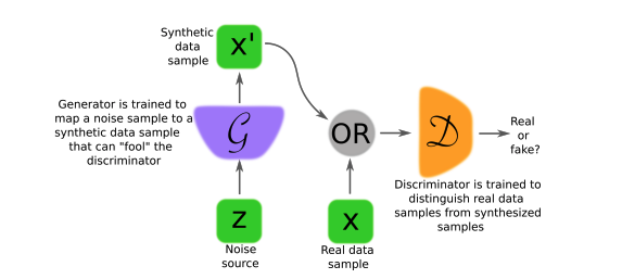
Diagram of a generative adversarial network. (Image source: https://arxiv.org/pdf/1710.07035.pdf)
Image to Image Translation
Image to image translation is a subfield of computer vision problems. The goal of such problems is to learn a mapping between an input and output image using paired training data. Most commonly, image to image translation is done using Convolutional Neural Networks to learn a parametric translation function from a dataset of input and output images. This allows users to generate a new image that has the same essential characteristics as an input image, but is in a different domain or style.
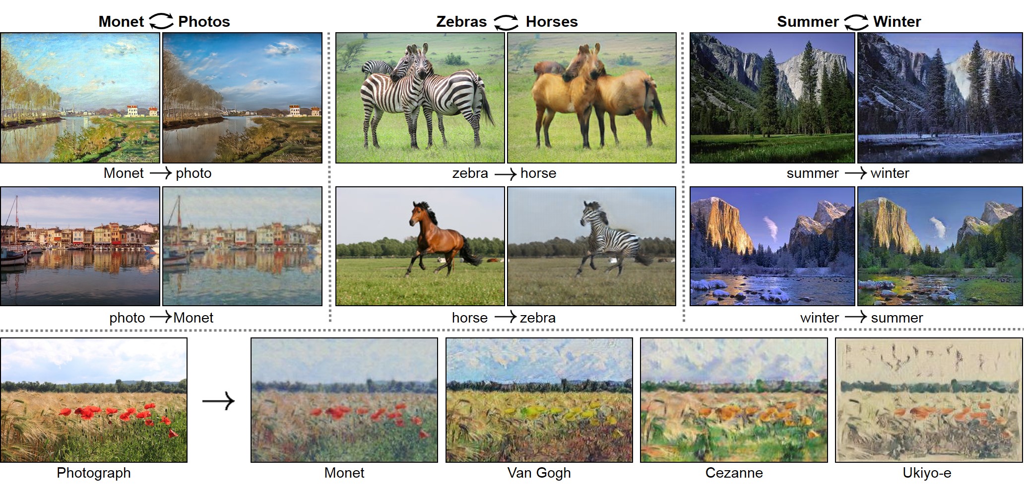
Image to image translation examples. (Image source: https://arxiv.org/pdf/1703.10593.pdf)
One drawback of such an approach however is that paired training data is not always available. For example, image pairs rarely exists for artistic stylization tasks due to the difficulty of generation: this requires skilled artists to craft artwork by hand.
Unpaired Image to Image Translation
An early technique to perform unpaired image to image translation was a Bayesian technique to determine the most likely output image. In this particular approach, P(X) is a patch-based Markov random field taken from the source image. The likelihood of the input is represented by a Bayesian network obtained from multiple style images.
CoGAN
In 2016, a Coupled GAN or CoGAN was proposed to learn a joint distribution of multi-domain images. CoGAN features a tuple of GAN’s for each image domain and uses a weight sharing constraint to learn a joint distribution for multi domain images.
As part of the study, CoGAN was used to generate faces with different attributes. The image below shows
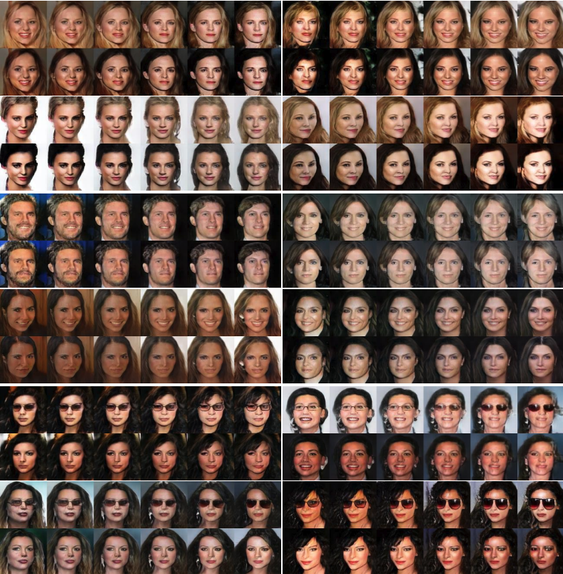
Pair face generation for blond-hair, smiling, and eyeglasses attributes. For each pair, the first row contains the faces with the attributes and the second row contains faces without the attributes. (Image source: https://arxiv.org/pdf/1606.07536.pdf)
Since at the time no models with the same capabilities existed, CoGAN was compared to a conditional GAN, which took a binary variable representing output domain as an input. When applied to specific tasks, CoGAN consistently outperformed the conditional GAN. One one task, CoGAN achieved accuracy of 0.952, while the conditional GAN has accuracy 0.909. On another task, CoGAN had accuracy 0.967 and the conditional GAN 0.778.
Most popular GANs
GANs have proven to be one of the most effective ways to generate Deep fakes. We will now perform an in depth analysis of three varieties of GANs: Cycle-GAN, Star-GAN, and Style-GAN.
Cycle-GAN Networks
The Cycle-GAN Networks devised in 2017 promised to perform image to image translation without paired examples. To do so, several assumptions needed to be made:
- There is an underlying relationship between the domains that must be learned
- Translation should be cycle consistent.
- The mapping is stochastic- probabilistic modeling is involved and there is some uncertainty in the output
The model is as follows:
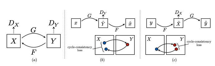
Cycle-GAN model. (Image source: https://arxiv.org/pdf/1703.10593.pdf)
A key component of Cycle-GANs is a DCGAN, which is a convolutional GAN whose generator and discriminator are both CNN’s for training stability purposes. The Cycle-GAN we will study uses two DCGAN’s, which means there are two generators and two discriminators.
Block diagrams of a generator and discriminator in a DGCAN are shown below:
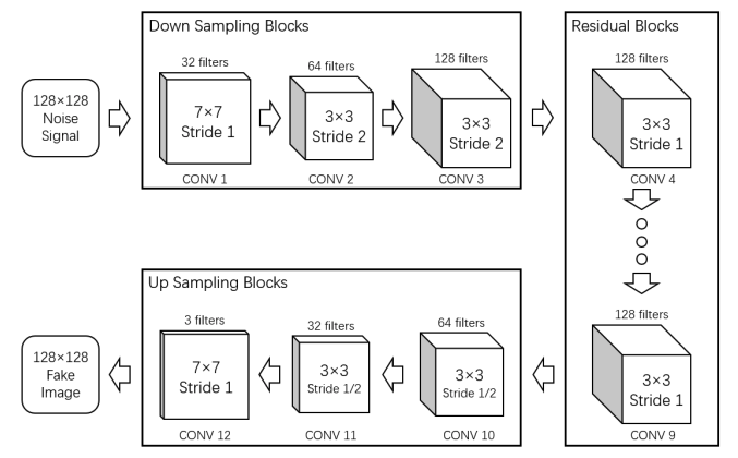
Block Diagram of a generator. (Image source: http://noiselab.ucsd.edu/ECE228_2018/Reports/Report16.pdf)
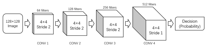
Block Diagram of a discriminator. (Image source: http://noiselab.ucsd.edu/ECE228_2018/Reports/Report16.pdf)
During training, the two DCGANs are sent different sets of images as inputs. We will use the following mathematical terminology:
- The model has two mapping functions: \(G : X \rightarrow Y\) and \(F : Y \rightarrow X\)
- \(X\) and \(Y\) are the domains for each respective DCGAN
- Input images \(x\) are members of domain \(X\) and input images \(y\) are members of domain \(Y\)
- The images generated in domain \(X\) should be similar to images in domain \(Y\) and vice versa
- The two generators are \(G\) and \(F\) and the respective discriminators are \(D_{y}\) and \(D_{x}\)
- Note the discriminator for generator \(G\) is \(D_{y}\) because we aim to differentiate between fake images \(G(x)\) and domain \(Y\)
- \(G(x)\) denotes images generated by \(G\) and \(F(y)\) denotes images generated by \(Y\)
Cycle-GAN Loss
Each DCGAN has two losses.
- We can combine both adversarial losses together to get:
- \[\mathcal{L}_{\mathrm{GAN}}=\mathbb{E}_{x \sim p_{\text {data }}(x)}\left[\left(1-D_Y(G(x))\right)^2\right] +\mathbb{E}_{y \sim p_{\text {data }}(y)}\left[\left(1-D_X(F(y))\right)^2\right]\]
- We can combine both discriminator losses together to get:
- \(\mathcal{L}_D=\mathbb{E}_{x \sim p_{\text {data }}(x)}\left[D_Y(G(x))^2\right] +\mathbb{E}_{y \sim p_{\text {data }}(y)}\left[D_X(F(y))^2\right]+\mathbb{E}_{x \sim p_{\text {data }}(x)}\left[\left(1-D_X(x)\right)^2\right] +\mathbb{E}_{y \sim p_{\text {data }}(y)}\left[\left(1-D_Y(y)\right)^2\right]\)
- \(\mathcal{L}_D=\mathbb{E}_{x \sim p_{\text {data }}(x)}\left[D_Y(G(x))^2\right] +\mathbb{E}_{y \sim p_{\text {data }}(y)}\left[D_X(F(y))^2\right]+\mathbb{E}_{x \sim p_{\text {data }}(x)}\left[\left(1-D_X(x)\right)^2\right] +\mathbb{E}_{y \sim p_{\text {data }}(y)}\left[\left(1-D_Y(y)\right)^2\right]\)
Cycle consistency losses or \(L_{cyc}\) are introduced to capture the assumption that the translation should be cycle consistent:
- Forward cycle consistency loss
- \[x \rightarrow G(x) \rightarrow F(G(x)) \approx x\]
- This formula refers to translating an impage \(x\) from domain \(X\) to domain \(Y\) via \(G\) and then back to domain \(X\) via \(F\)
- Backward cycle consistency loss
- \[y \rightarrow F(y) \rightarrow G(F(y)) \approx y\]
- This formula refers to translating an impage \(y\) from domain \(Y\) to domain \(X\) via \(F\) and then back to domain \(Y\) via \(G\)
- Total cycle consistency loss
- \[\mathcal{L}_{\text {cyc }}=\mathbb{E}_{x \sim p_{\text {data }}(x)}\left[\|F(G(x))-x\|_1\right] +\mathbb{E}_{y \sim p_{\text {data }}(y)}\left[\|G(F(y))-y\|_1\right]\]
- The corresponding example code where \(A\) is \(X\) and \(B\) is \(Y\) is as follows:
# GAN loss D_A(G_A(A))
self.loss_G_A = self.criterionGAN(self.netD_A(self.fake_B), True)
# GAN loss D_B(G_B(B))
self.loss_G_B = self.criterionGAN(self.netD_B(self.fake_A), True)
# Forward cycle loss || G_B(G_A(A)) - A||
self.loss_cycle_A = self.criterionCycle(self.rec_A, self.real_A) * lambda_A
# Backward cycle loss || G_A(G_B(B)) - B||
self.loss_cycle_B = self.criterionCycle(self.rec_B, self.real_B) * lambda_B
# combined loss and calculate gradients
self.loss_G = self.loss_G_A + self.loss_G_B + self.loss_cycle_A + self.loss_cycle_B + self.loss_idt_A + self.loss_idt_B
self.loss_G.backward()
We can also introduce the \(L_{identity}\) loss. This preserves color composition between inputs and output.
- \[\mathcal{L}_{\text {identity }}=\mathbb{E}_{y \sim p_{\text {data }}(y)}\left[\|G(y)-y\|_1\right] +\mathbb{E}_{x \sim p_{\text {data }}(x)}\left[\|F(x)-x\|_1\right]\]
- The corresponding example code where \(A\) is \(X\) and \(B\) is \(Y\) is as follows:
# Identity loss
  if lambda_idt > 0:
      # G_A should be identity if real_B is fed: ||G_A(B) - B||
      self.idt_A = self.netG_A(self.real_B)
      self.loss_idt_A = self.criterionIdt(self.idt_A, self.real_B) * lambda_B * lambda_idt
      # G_B should be identity if real_A is fed: ||G_B(A) - A||
      self.idt_B = self.netG_B(self.real_A)
      self.loss_idt_B = self.criterionIdt(self.idt_B, self.real_A) * lambda_A * lambda_idt
  else:
      self.loss_idt_A = 0
      self.loss_idt_B = 0
We can create the total generator loss as follows:
\(\mathcal{L}_G=\lambda_1 \mathcal{L}_{\mathrm{GAN}}+\lambda_2 \mathcal{L}_{\text {identity }}+\lambda_3 \mathcal{L}_{\text {cyc }}\)
Note: \(\lambda_1\), \(\lambda_2\), and \(\lambda_3\) control the relative importances of the various losses.
We can also split the discriminator loss as well:
- \[\mathcal{L}_{D_X}=\mathbb{E}_{x \sim p_{\text {data }}(x)}\left[\left(1-D_X(x)\right)^2\right] +\mathbb{E}_{y \sim p_{\text {data }}(y)}\left[D_X(F(y))^2\right]\]
- \[\mathcal{L}_{D_Y}=\mathbb{E}_{y \sim p_{\text {data }}(y)}\left[\left(1-D_Y(y)\right)^2\right] +\mathbb{E}_{x \sim p_{\text {data }}(x)}\left[D_Y(G(x))^2\right]\]
- The corresponding example code where \(A\) is \(X\) and \(B\) is \(Y\) is as follows:
def backward_D_A(self):
    """Calculate GAN loss for discriminator D_A"""
    fake_B = self.fake_B_pool.query(self.fake_B)
    self.loss_D_A = self.backward_D_basic(self.netD_A, self.real_B, fake_B)

def backward_D_B(self):
    """Calculate GAN loss for discriminator D_B"""
    fake_A = self.fake_A_pool.query(self.fake_A)
    self.loss_D_B = self.backward_D_basic(self.netD_B, self.real_A, fake_A)
In each epoch \(\mathcal{L}_G\) is calculated and backpropogated. Next, \(\mathcal{L}_{D_X}\) is calculated and backpropogated. Lastly, \(\mathcal{L}_{D_Y}\) is calculated and backpropogated.
Colab Notebook Results
Here is an image translation we ran where we translated a picture of the UCLA campus to the domain of a Monet painting.
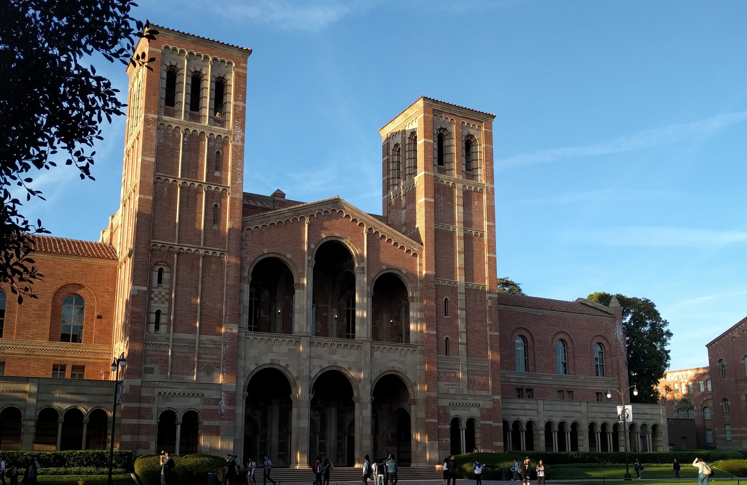
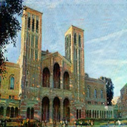
Results generated from our colab notebook.
You can see that CycleGAN can perform domain to domain translation well.
StarGAN
An enhanced GAN variation, StarGAN, was proposed in 2018. StarGAN performs image-to-image translations for multiple domains with only a single model; this allows a single network to simultaneously train multiple datasets with different domains. There is some important terminology to keep in mind when discussing the StarGAN: attribute refers to an inherent meaningful feature such as hair color or gender, attribute value is the value of an attribute, for example, male/female for gender, and a domain is a set of images with the same attribute value.
The availability of datasets such as CelebA, which contain facial attribute labels, allow us to change images according to attributes from multiple domains, a task called multi-domain-image-to-image translation. An example showing the CelebA dataset translated according to the domains blond hair, gender, age, and pale skin is as follows:
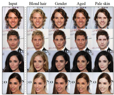
Multi-domain image-to-image translation results on the CelebA dataset via transferring knowledge learned from the RaFD dataset. (Image source: https://arxiv.org/pdf/1711.09020.pdf)
An issue with existing models is the inefficiency when performing such multi-domain image tasks. This is where StarGAN outperformed existing models of the time. StarGAN uses a single generator to learn mappings between \(k\) domains, as opposed to the previous \(k(k-1)\) generators needed.
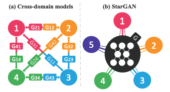
Comparison between cross-domain models and StarGAN. (Image source: https://arxiv.org/pdf/1711.09020.pdf)
StarGAN works as follows. The generator \(G\) takes the image \(x\) and domain information as inputs and learns to translate the image into the specified domain \(c\), which is randomly generated during training. The domain information is represented as a binary or one-hot vector label. By adding a mask vector to the domain label, we can also enable join training between domains of different datasets. The discriminator \(D\) creates probability distributions over both sources and domain labels: \(D: x \rightarrow\left\{D_{s r c}(x), D_{c l s}(x)\right\}\). An overview of the StarGAN model is shown below.
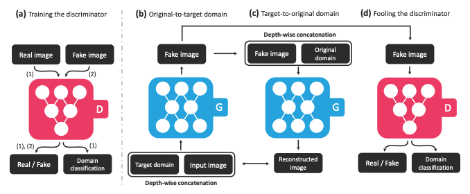
“(a) D learns to distinguish between real and fake images and classify the real images to its corresponding domain. (b) G takes in as input both the image and target domain label and generates an fake image. The target domain label is spatially replicated and concatenated with the input image. (c) G tries to reconstruct the original image from the fake image given the original domain label. (d) G tries to generate images indistinguishable from real images and classifiable as target domain by D.” (Image source: https://arxiv.org/pdf/1711.09020.pdf)
StarGAN Loss
There are several losses involved in StarGAN.
Adversarial Loss is used to make the generated images indistinguishable from real images. In the equation below, \(G(x, c)\) is the image generated by \(G\). Furthermore, \(G\) tries to minimize \(D_{s r c}\) while \(D\) tries to maximize this.
\(\mathcal{L}_{a d v}= \mathbb{E}_x\left[\log D_{s r c}(x)\right]+ \mathbb{E}_{x, c}\left[\log \left(1-D_{s r c}(G(x, c))\right)\right]\)
The domain classification loss is introduced to ensure good classification performance. It is used when optimizing both \(G\) and \(D\) and can be separated into two terms.
-
Domain classification loss of fake images used to optimize G: \(\mathcal{L}_{c l s}^f=\mathbb{E}_{x, c}\left[-\log D_{c l s}(c \mid G(x, c))\right]\)
-
Domain classification loss of real images used to optimize D: \(\mathcal{L}_{c l s}^r=\mathbb{E}_{x, c^{\prime}}\left[-\log D_{c l s}\left(c^{\prime} \mid x\right)\right]\)
- \(D_{c l s}\left(c^{\prime} \mid x\right)\) represents a probability distribution over domain labels computed by D
- \(D_{c l s}\left(c^{\prime} \mid x\right)\) represents a probability distribution over domain labels computed by D
Lastly, the reconstruction loss is a cycle consistency loss applied to ensure that translated images only change the domain-related parts of the input while preserving the remaining content of their input images.
\(\mathcal{L}_{r e c}=\mathbb{E}_{x, c, c^{\prime}}\left[\left\|x-G\left(G(x, c), c^{\prime}\right)\right\|_1\right]\)
The combined loss functions for StarGAN are as follows:
- \[\mathcal{L}_D= -\mathcal{L}_{adv} + \lambda_{cls} \mathcal{L}_{cls}^r\]
- \[\mathcal{L}_G= \mathcal{L}_{adv} + \lambda_{cls} \mathcal{L}_{cls}^r + \lambda_{rec} \mathcal{L}_{rec}\]
Where \(\lambda_{cls}\) and \(\lambda_{rec}\) are hyperparameters (in this experiment they are set to 1 and 10 respectively).
The code snippet defining \(\mathcal{L}_D\):
# Compute loss with real images.
out_src, out_cls = self.D(x_real)
d_loss_real = - torch.mean(out_src)
d_loss_cls = self.classification_loss(out_cls, label_org, self.dataset)

# Compute loss with fake images.
x_fake = self.G(x_real, c_trg)
out_src, out_cls = self.D(x_fake.detach())
d_loss_fake = torch.mean(out_src)

# Compute loss for gradient penalty.
alpha = torch.rand(x_real.size(0), 1, 1, 1).to(self.device)
x_hat = (alpha * x_real.data + (1 - alpha) * x_fake.data).requires_grad_(True)
out_src, _ = self.D(x_hat)
d_loss_gp = self.gradient_penalty(out_src, x_hat)

# Backward and optimize.
d_loss = d_loss_real + d_loss_fake + self.lambda_cls * d_loss_cls + self.lambda_gp * d_loss_gp
self.reset_grad()
d_loss.backward()
self.d_optimizer.step()
The code snippet defining \(\mathcal{L}_G\):
if (i+1) % self.n_critic == 0:
  # Original-to-target domain.
  x_fake = self.G(x_real, c_trg)
  out_src, out_cls = self.D(x_fake)
  g_loss_fake = - torch.mean(out_src)
  g_loss_cls = self.classification_loss(out_cls, label_trg, self.dataset)

  # Target-to-original domain.
  x_reconst = self.G(x_fake, c_org)
  g_loss_rec = torch.mean(torch.abs(x_real - x_reconst))

  # Backward and optimize.
  g_loss = g_loss_fake + self.lambda_rec * g_loss_rec + self.lambda_cls * g_loss_cls
  self.reset_grad()
  g_loss.backward()
  self.g_optimizer.step()
StarGAN v2
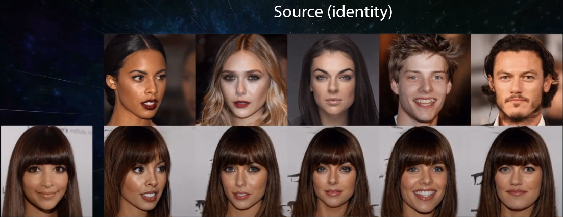
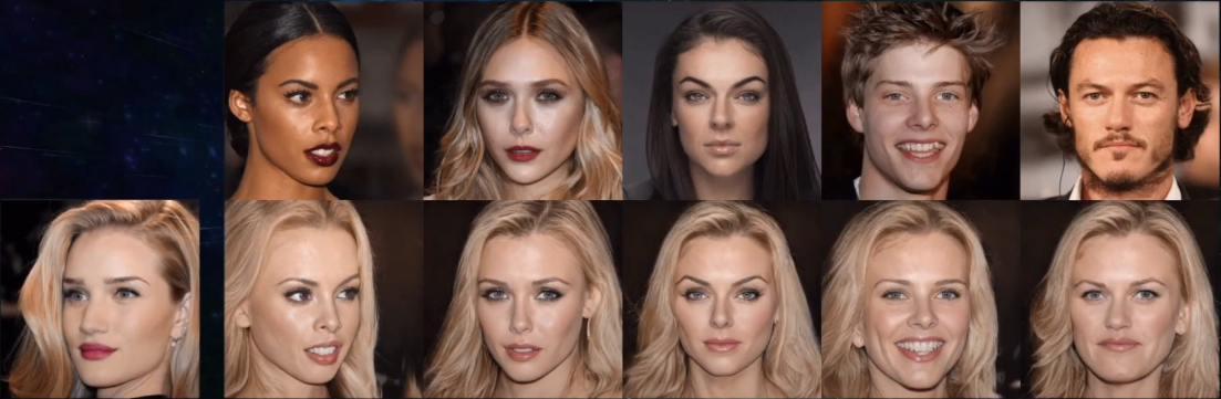
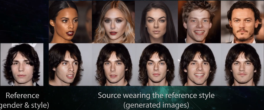
“StarGAN v2: Diverse Image Synthesis for Multiple Domains.” (Image source: https://arxiv.org/pdf/1912.01865.pdf
StarGAN v2 expands upon the work done with StarGAN to allow for the model to learn a mapping which captures the multi-modal nature of the data distribution. This allows for the generation of diverse images across multiple domains. A key change from StarGAN is the switch form the domain label to domain specific style code which represents diverse styles of a specific domain. This is done by introducing a mapping network, which learns to transform random Gaussian noise into a style code, and a style encoder, which learns to extract the style code from a given image. The generator \(G\) translates input image \(x\) into output \(G(x,s)\) where \(s\) is the domain specific style code. The discriminator \(D\) is multi-task and has several output branches.
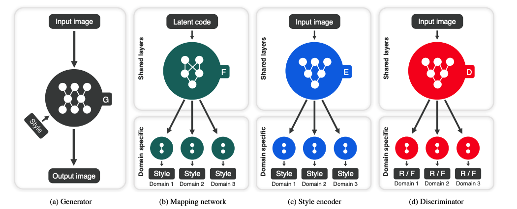
“Overview of StarGAN v2, consisting of four modules. (a) The generator translates an input image into an output image reflecting the domain-specific style code. (b) The mapping network transforms a latent code into style codes for multiple domains, one of which is randomly selected during training. (c) The style encoder extracts the style code of an image, allowing the generator to perform referenceguided image synthesis. (d) The discriminator distinguishes between real and fake images from multiple domains. Note that all modules except the generator contain multiple output branches, one of which is selected when training the corresponding domain.” (Image source: https://arxiv.org/pdf/1912.01865.pdf)
StarGANv2 Loss
Similar to the original StyleGAN, version 2 comines several specific loss functions.
The adversarial loss again is used to ensure that the generated images are indistinguishable from the real images.
\[\mathcal{L}_{a d v}= \mathbb{E}_{\mathbf{x}, y}\left[\log D_y(\mathbf{x})\right]+ \mathbb{E}_{\mathbf{x}, \widetilde{y}, \mathbf{z}}\left[\log \left(1-D_{\tilde{y}}(G(\mathbf{x}, \widetilde{\mathbf{s}}))\right)\right]\]The appropriate code is as follows:
def adv_loss(logits, target):
  assert target in [1, 0]
  targets = torch.full_like(logits, fill_value=target)
  loss = F.binary_cross_entropy_with_logits(logits, targets)
  return loss
Style reconstruction loss is needed to enforce generator \(G\) to utilize the style code \(\widetilde{s}\). The major difference with this method is that a single encoder \(E\) is trained to encourage diverse outputs for multiple domains. \(E\) then permits \(G\) to reflect the style of a reference image at test time.
\[\mathcal{L}_{s t y}= \mathbb{E}_{\mathbf{x}, \widetilde{y}, \mathbf{z}}\left[\left\|\widetilde{\mathbf{s}}-E_{\widetilde{y}}(G(\mathbf{x}, \widetilde{\mathbf{s}}))\right\|_1\right]\]The appropriate code is as follows:
# style reconstruction loss
s_pred = nets.style_encoder(x_fake, y_trg)
loss_sty = torch.mean(torch.abs(s_pred - s_trg))
Style diversification includes regularizing \(G\) with diversity sensitive loss to allow the generator to produce diverse images.
\[\mathcal{L}_{d s}= \mathbb{E}_{\mathbf{x}, \widetilde{y}, \mathbf{z}_1, \mathbf{z}_2}\left[\left\|G\left(\mathbf{x}, \widetilde{\mathbf{s}}_1\right)-G\left(\mathbf{x}, \widetilde{\mathbf{s}}_2\right)\right\|_1\right]\]The appropriate code is as follows:
# diversity sensitive loss
if z_trgs is not None:
    s_trg2 = nets.mapping_network(z_trg2, y_trg)
else:
    s_trg2 = nets.style_encoder(x_ref2, y_trg)
x_fake2 = nets.generator(x_real, s_trg2, masks=masks)
x_fake2 = x_fake2.detach()
loss_ds = torch.mean(torch.abs(x_fake - x_fake2))
We then introduce a cycle consistency loss to ensure that the generated image \(G(\mathbf{x}, \widetilde{\mathbf{s}})\) preserves the original properties (non related to style) of its input image.
\[\mathcal{L}_{c y c}= \mathbb{E}_{\mathbf{x}, y, \widetilde{y}, \mathbf{z}}\left[\|\mathbf{x}-G(G(\mathbf{x}, \widetilde{\mathbf{s}}), \hat{\mathbf{s}})\|_1\right]\]The appropriate code is as follows:
# cycle-consistency loss
masks = nets.fan.get_heatmap(x_fake) if args.w_hpf > 0 else None
s_org = nets.style_encoder(x_real, y_org)
x_rec = nets.generator(x_fake, s_org, masks=masks)
loss_cyc = torch.mean(torch.abs(x_rec - x_real))
The overall loss can be represented as follows:
\[\min _{G, F, E} \max _D \mathcal{L}_{a d v}+\lambda_{s t y} \mathcal{L}_{s t y} -\lambda_{d s} \mathcal{L}_{d s}+\lambda_{c y c} \mathcal{L}_{c y c}\]where \(\lambda_{s t y}\), \(\lambda_{d s}\), and \(\lambda_{c y c}\) are hyperparameters.
The appropriate code is as follows:
loss = loss_adv + args.lambda_sty * loss_sty - args.lambda_ds * loss_ds + args.lambda_cyc * loss_cyc
Colab Notebook Results
Here is an animation showing image generation using the input images of our faces, the professor’s face, and our TA’s face.
Results generated from our colab notebook.
You can see that the domain translation comes out well overall. However, small details make some translations unrealistic, such as a portion of a pair of glasses on a face or misaligned features.
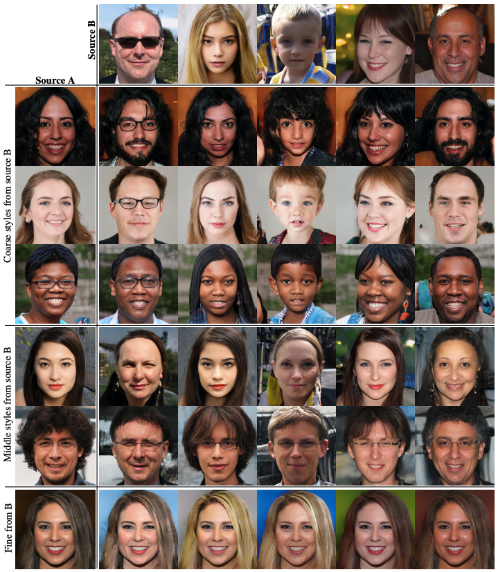
StyleGAN
Another recently proposed model is StyleGAN, which is based on style transfer principles. StyleGAN proposes changes to the traditional GAN architecture which include the introduction of a mapping network that maps points in latent space to an intermediate latent space, which is used to control style at every point in the generator model. Stylegan also uses noise as a source of variation at every point in the generator model.
“StyleGAN Demo.” (Image source: https://arxiv.org/pdf/1812.04948.pdf)
Style Based Generator
In traditional GANs, the input layer provides the latent code to the generator. In StyleGAN however, we omit the first layer and use a learned constant \(w\) instead. StyleGAN also uses AdaIN, or adaptive instance normalization, to control the generator at each convolution layer. AdaIN takes in an input \(x\) and style \(y\) and aligns the channel wise mean and variance of \(x\) to match that of \(y\). AdaIN has to learnable affine parameters and instead adaptively computes the affine parameters from \(y\). The AdaIN equation is as follows: \(\operatorname{AdaIN}\left(\mathbf{x}_i, \mathbf{y}\right)=\mathbf{y}_{s, i} \frac{\mathbf{x}_i-\mu\left(\mathbf{x}_i\right)}{\sigma\left(\mathbf{x}_i\right)}+\mathbf{y}_{b, i}\)
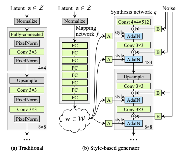
“Traditional generator vs StyleGAN. \(W\) is the intermediate latent space, \(A\) is a learned affine transform, and \(B\) applies learned scaling factors to the noise input for each channel. This generator has 26.2M trainable parameters, while a standard generator has 23.1M trainable parameters.” (Image source: https://arxiv.org/pdf/1812.04948.pdf)
StyleGAN does not modify the traditional loss functions used by GAN. When Frechet inception distance (FID), a metric used to assess the quality of images created by GANs, is analyzed, the benefits are clear to see.
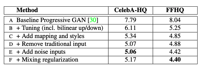
“FID for various generator designs. The FIDs for this paper were calculated by drawing 50,000 random images from the training set and reporting the lowest distance found during training. Note: lower FID is better.” (Image source: https://arxiv.org/pdf/1812.04948.pdf)
The quality of generated images using StyleGAN was improved due to several key changes.
- Introducing bilinear up and downsampling operations, longer training, and tuned hyperparameters
- Adding the mapping network and AdaIN operations
- Removing the input layer and starting image synthesis from a learned tensor
- Noise inputs (see figure below for visualizations of effect)
- Mixing regularization, which entails using two random latent codes instead of one during training for a subset of images.
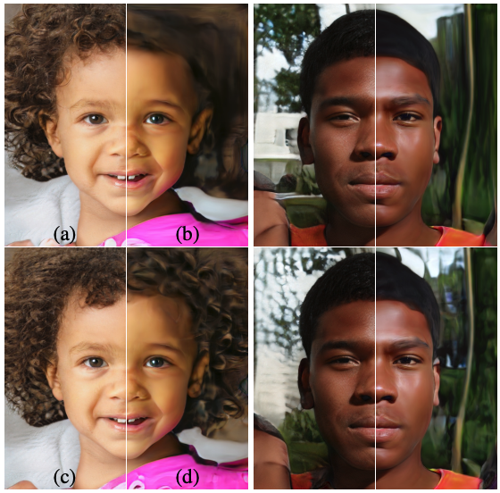
“Noise input effects. In (a) noise is applied to all layers. In (b) there is no noise. In (c) there is noise in fine layers only and in (d) there is noise in course layers only.” (Image source: https://arxiv.org/pdf/1812.04948.pdf)
Overall, we can see that no noise results in a featureless look, coarse noise results in hair curling and bigger background features, and fine noise results in finer detail in the hair, skin, and background.
StyleGAN v3
In October 2021, version 3 of StyleGAN, or AliasFreeGAN, was announced. The main benefit of this version was the ability to fix the “texture sticking” issue that occurred when morphing from one face to another face. In the animation below, you can see that the features on the left appear to be sticking to the screen rather than the face.
“Demo of v3 changes.” (Image source: https://nvlabs.github.io/stylegan3/)
The overall design is as follows:
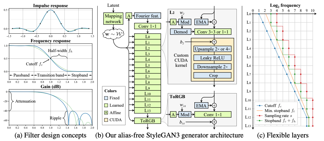
“(a) 1D example of a 2× upsampling filter (b) Alias-free generator, the main datapath consists of Fourier features and normalization, modulated convolutions, and filtered nonlinearities (c) Flexible layer specifications.” (Image source: https://arxiv.org/pdf/2106.12423.pdf)
Colab Notebook Results
Here is an animation showing image generation using StyleGAN v3.
Results generated from our colab notebook.
You can see that the domain translation comes out very cleanly. The images transition very smoothly and texture sticking is not an issue.
Comparisons and Conclusions
Now that we have explored the topics of CycleGAN, StarGAN, and StyleGAN, let’s take a look at the similarities and differences between these three classes of generative adversarial networks.
With the purpose of image synthesis and manipulation, all three types of models share a similar GAN architecture with a generator that creates images and a discriminator that evaluates the generated images’ quality. The generator and discriminator compete against each other in a minimax game, improving each other’s performance during training.
In addition, all the models use adversarial loss to ensure that the generated images are indistinguishable from real images in the target domain. The discriminator’s goal is to correctly classify real and fake images, while the generator’s goal is to create images that the discriminator cannot distinguish from real ones.
Despite a shared architectural DNA, each model has its own strengths and weaknesses that distinguish it from the others.
- CycleGAN is composed of 2 GANs, making it a total of 2 generators and 2 discriminators. Given two distinct sets of images from different domains, CycleGAN learns to translate images from one domain to another without requiring paired examples during its training or testing stage. But this ability to map between the input and output domain is deterministic in nature, resulting in the model learning one-to-one mappings. One-to-one mapping leads to a lack of diversity in the translated images which does not represent the fact that “most relationships across domains are more complex and better characterized as many-to-many.” When the model is given more complex cross-domain relationships, it fails to capture the true structured conditional distribution and results in an arbitrary one-to-one mapping. For example, CycleGAN struggles to learn that an image of a sunny scene could be translated into a cloudy or rainy scene.
- StarGAN uses a single generator and a single discriminator to perform image translation between multiple domains and unlike CycleGAN, it learns many-to-many mappings. In addition to adversarial loss, it also utilizes domain classification loss and reconstruction loss. One weakness of StarGAN may come from its single generator and discriminator structure. This limited capacity can prevent it from learning complex mappings among numerous domains. This can sometimes result in unwanted attributes in the generated images as it is difficult to learn to disentangle specific features that may be correlated.
- StyleGAN generates the most highly realistic and high-resolution images out of all three models. It contains a generator, consisting of a mapping network, an adaptive instance normalization (AdaIN) layer, and a synthesis network, in addition to a discriminator. Producing these high-quality images can require a more complex and resource intensive training process due to the model’s approach of progressive growing and style mixing. It also suffers from other common GAN weaknesses such as mode collapse.
Demo Links
The link to our Google Colaboratory demo can be found here and our Drive Folder with results and our overview video can be found here. The results from our code can be found in the drive folder and our video overview covers the results as well.
References
[1] Shen, Tianxiang, et al. ““Deep Fakes” using Generative Adversarial Networks (GAN).” University of California, San Diego. 2018.
[2] Ren, Yurui, et al. “Deep Image Spatial Transformation for Person Image Generation.” Proceedings of the IEEE conference on computer vision and pattern recognition. 2020.
[3] Creswell, Antonia, et al. “Generative Adversarial Networks: An Overview.” Proceedings of the IEEE conference on computer vision and pattern recognition. 2017.
[4] Zhu, Jun-Yan, et al. “Unpaired Image-to-Image Translation using Cycle-Consistent Adversarial Networks.” Proceedings of the International Conference on Computer Vision. 2017.
[5] Rosales, Rómer, et al. “Unsupervised image translation.” Proceedings of the International Conference on Computer Vision. 2003.
[6] Yu, Ming-Yu, et al. “Coupled Generative Adversarial Networks.” Proceedings of the Conference on Neural Information Processing Systems. 2016.
[7] Choi, Yunjey, et al. “StarGAN: Unified Generative Adversarial Networks for Multi-Domain Image-to-Image Translation.” Proceedings of the IEEE conference on computer vision and pattern recognition. 2018.
[8] Choi, Yunjey, et al. “StarGAN v2: Diverse Image Synthesis for Multiple Domains.” Proceedings of the IEEE conference on computer vision and pattern recognition. 2020.
[9] Karras, Tero, et al. “A Style-Based Generator Architecture for Generative Adversarial Networks.” Proceedings of the IEEE conference on computer vision and pattern recognition. 2019.
[10] Karras, Tero, et al. “A Style-Based Generator Architecture for Generative Adversarial Networks.” Proceedings of the IEEE conference on computer vision and pattern recognition. 2019.
[11] Xun, Huang, et al. “Arbitrary Style Transfer in Real-time with Adaptive Instance Normalization.” Proceedings of the International Conference on Computer Vision. 2017.
[12] Karras, Tero, et al. “Alias-Free Generative Adversarial Networks.” Proceedings of the Conference on Neural Information Processing Systems. 2021.