Generating Images with Diffusion Models
This project explores the latest technology behind Image-generative AIs such as DALLE-2 and Imagen. Specifically we’ll be going over the research and techniques behind Diffusion Models, and a toy implementation in Pytorch/COLAB.
- 10 Minute Spotlight Presentation
- What are diffusion models?
- CelebA Dataset
- 1. The Forward Diffusion Process
- 2. The Reverse Diffusion Process
- Generating Random Images
- Comparisons to VAE and GAN
- Further Exploration: Conditional Image Generation with Diffusion Models
- COLAB Notebook
- References
10 Minute Spotlight Presentation
Youtube Link Link to Notebook at bottom.
What are diffusion models?
Diffusion models are a popular way to generate new images that are of a similar type to the training data. The diffusion technique is found in Dall-E, Lensa, and more! The strategy behind diffusion models is to gradually destroy the training images by adding noise, and then recovering the image by learning how to remove noise. By learning this recovery process using a neural network, we can generate new images by applying the recovery process to random noise.
There are two main parts to training diffusion models. The first part is adding noise(typically, Gaussian noise). In each “step”, we add more noise to the image, so timestep 2 is noisier than timestep one. The more steps we have the better the model tends to be, since having more steps means that the steps are smaller and in the denoising process, it is easier for the model to remove a little noise than to remove a lot of noise. The second part is to train a neural network that given some timestep, can recover a previous timestep. For this “backwards” process, we need to have timestep encoding since we will have the same model for all timesteps, and we need to define a loss function so that we can improve our model with gradient descent.
Once we know how to recover a previous timestep from some timestep, our model is now generative. We start with random noise and go “backwards” timestep by timestep until we get a new image!
While diffusion models these days include many advanced optimizations and features, we will focus on a relatively simple implementation that focuses on the core parts.
CelebA Dataset
For the purposes of exploring diffusion models, our project focuses on the CelebA faces dataset. This dataset is a collection of 20,000 images of celebrity faces. After resizing these images to 64x64, our goal in our Google Colab notebook is to implement diffusion models to regenerate the faces. The implementation of our Notebook and the discussion of topics in this article rely heavily on the founding papers of diffusion models: “Denoising Diffusion Probabilistic Models”, “Diffusion Models Beat GANs on Image Synthesis.” The GitHub repositories of these papers will also be cited at the end of this article.
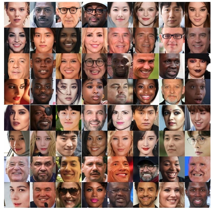
Fig. CelebA Faces Dataset.
1. The Forward Diffusion Process
The forward process of the diffusion model involves adding noise to an image. This is done by adding noise to each of the three channels(r, g, b) of each pixel. In this diffusion model, we add Gaussian noise, which is noise that has a normal(or Gaussian) distribution. Gaussian noise has two parameters, the mean and the standard deviation. We usually set the mean to 0 and the standard deviation is determined by a scheduler whose input is the timestep.
For a given timestep, you can find the next timestep by applying gaussian noise as described above. This means that each timestep directly depends only on the previous timestep, forming a Markov chain. The equation to go from one node of the markov chain to the next of this Markov chain is as follows:
\[q\left(x_t \mid x_{t-1}\right)=N\left(x_t ; \sqrt{1-\beta_t} x_{t-1}, \beta_t I\right)\]Based on the fact that each state depends on the previous state, and the previous state depends on its previous state, we can use Bayesian probability to obtain a closed form:
\[q\left(x_{1: T} \mid x_0\right)=\prod_{t=1}^T q\left(x_t \mid x_{t-1}\right)\]To compute some timestep, we still have to compute all the previous timesteps which is very inefficient. So, we use a reparameterization trick to obtain a form that allows us to obtain any time step directly from the original image.
\[\mathbf{x}_t \sim q\left(\mathbf{x}_t \mid \mathbf{x}_0\right)=\mathcal{N}\left(\mathbf{x}_t ; \sqrt{\bar{\alpha}_t} \mathbf{x}_0,\left(1-\bar{\alpha}_t\right) \mathbf{I}\right)\]This allows us to find a timestep without finding all of the previous timesteps which allows us to very efficiently calculate the loss between predicted timestep and actual timestep.
def forward_diffusion_sample(x_0, t, device="cpu"):
    """
    Takes an image and a timestep as input and
    returns the noisy version of it
    """
    noise = torch.randn_like(x_0)
    sqrt_alphas_cumprod_t = get_index_from_list(sqrt_alphas_cumprod, t, x_0.shape)
    sqrt_one_minus_alphas_cumprod_t = get_index_from_list(
        sqrt_one_minus_alphas_cumprod, t, x_0.shape
    )
    # mean + variance
    return sqrt_alphas_cumprod_t.to(device) * x_0.to(device) \
    + sqrt_one_minus_alphas_cumprod_t.to(device) * noise.to(device), noise.to(device)
There are different ways to schedule noise(how standard deviation(beta) is calculated), such as cosine, quadratic or setting it to a constant. In this demo, we used a linear schedule which means beta is a linear function of the timestep. The larger the standard deviation of the noise, the faster we converge to a mean of 0(pure 0) which means that large beta corrupts the image faster. The linear schedule of the noise means that we add more noise at later time steps than we do so in earlier timesteps.
def linear_beta_schedule(timesteps, start=0.0001, end=0.02):
    return torch.linspace(start, end, timesteps)
This is an example of adding noise to an image in the dataset.
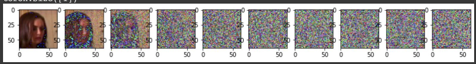
Fig. Example of Forward Diffusion Process.
2. The Reverse Diffusion Process
Now that we’ve generated samples of images with gaussian noise added according to a beta scheduler, we have to design our Neural Network to recover the original image given a noisy image. To do this, we must generate the probability distribution of noise pixels across the image. The goal of this is to learn the mean of the Gaussian distributions that were used to generate the noise at each timestep during the forward-diffusion process. Below is the math from the literature which describes this behavior. We want to predict the t - 1 timestep from the t timestep
\[p_\theta\left(\mathbf{x}_{0: T}\right)=p\left(\mathbf{x}_T\right) \prod_{t=1}^T p_\theta\left(\mathbf{x}_{t-1} \mid \mathbf{x}_t\right)\] \[p_\theta\left(\mathbf{x}_{t-1} \mid \mathbf{x}_t\right)=\mathcal{N}\left(\mathbf{x}_{t-1} ; \boldsymbol{\mu}_\theta\left(\mathbf{x}_t, t\right), \mathbf{\Sigma}_\theta\left(\mathbf{x}_t, t\right)\right)\]In implementation we use the UNet model, named as such because of the shape of the architecture. Particularly, UNet models have the unique property of equal input and output dimensions. The UNet model convolutes the image down to a very deep and small representation, and then does reverse convolutions to restore the image to its original dimensions. These are referred to as downsampling and upsampling respectively. The architecture of this model is great for problems that require more than a single image classification. In our case, we aim to predict the noise of a single time step given a noisy image. Specifically, given a noisy image of dimensions (C, H, W) we want to predict an equivalently sized (C, H, W) image that represents the noise of each pixel. By doing so we can subtract the noise from the noisy image and reverse a single step of the forward diffusion process.
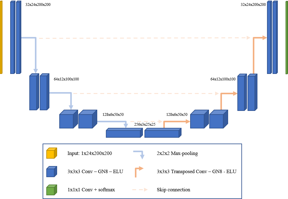
Fig. U-Net Architecture.
# Initial projection
self.conv0 = nn.Conv2d(image_channels, down_channels[0], 3, padding=1)

# Downsample blocks
self.downs = nn.ModuleList([Block(down_channels[i], down_channels[i+1], \
                            time_emb_dim) \
            for i in range(len(down_channels)-1)])
# Upsample blocks
self.ups = nn.ModuleList([Block(up_channels[i], up_channels[i+1], \
                                time_emb_dim, up=True) \
            for i in range(len(up_channels)-1)])

self.output = nn.Conv2d(up_channels[-1], 3, out_dim)
Attached is a code snippet of our UNet architecture which contains several layers. The first and last are initial and final convolutional layers that wrap our UNet. The UNet itself contains a module list of downsample blocks followed by a module list of upsample blocks. Each block is a convolutional layer with a timestep encoding concatenated with the input.
The neural network has shared parameters across time meaning that it is unable to distinguish between different timesteps of the reverse diffusion process. For example, it can’t distinguish between t = 100 or t = 8, determining how much current noise is in the image. To combat this problem, we introduce timestep encodings/embeddings which are taken from the positional embeddings that we see in transformers. We’ve seen this type of positional embedding in models like BERT in NLP and ViT in computer vision. Positional embeddings can be visualized as such where each timestep would have a unique embedding. We append this timestep embedding before feeding the input to each block within our downsample and upsample module lists.
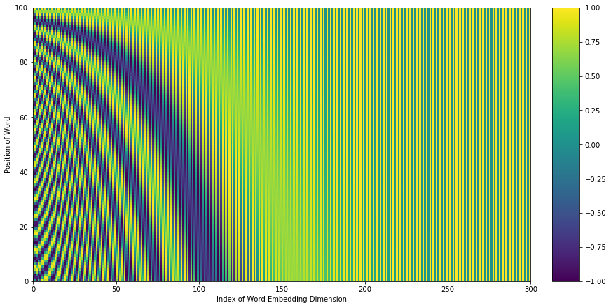
Fig. Position Encoding Graph.
The last detail of the model is the loss functions, which dictates the way the parameters of the model are trained. In our case, we simply take the L1 or L2 distance between the prediction of our noise image and the actual noise image that was added for the image. In implementation, we simply use the forward diffusion process we designed earlier to generate the actual noise.
def get_loss(model, x_0, t):
    x_noisy, noise = forward_diffusion_sample(x_0, t, device)
    noise_pred = model(x_noisy, t)
    return F.l1_loss(noise, noise_pred)
After training for several epochs, here are some examples of generated images. The faces on the left are all generated faces from our Diffusion Model. As you can see the faces aren’t perfect (given the limited training time/resources), but they are very recognizable with full facial features.
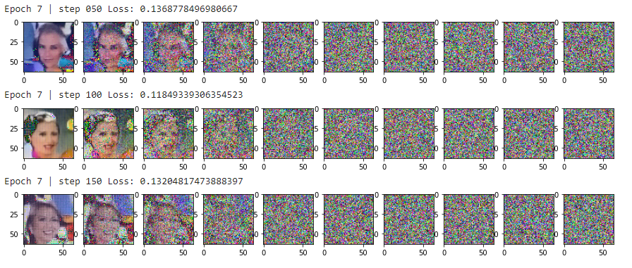
Fig. Training Results.
Generating Random Images
Once the model is fully trained, it is relatively simple for our model to generate noise. All you need is to generate random noise in the dimensions of the training data, and run that noise through the UNet we trained earlier. The UNet will perform the reverse diffusion process, removing some noise from the random image at each time step. At the end of the reverse diffusion process, we have a perfectly random-generated celebrity face.
Comparisons to VAE and GAN
Generative Adversarial Networks and Variational Autoencoders were both previous alternatives to doing image generation. With the release of technologies such as DALLE-2, we now see the fascinating power of diffusion models for generating images. How do these three compare?
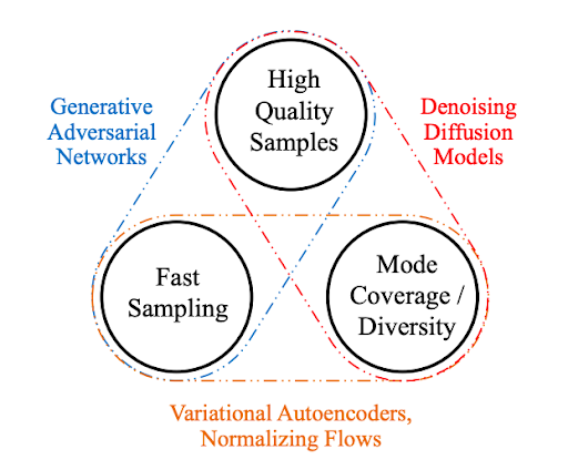
Fig. Comparison to GAN and VAE.
GANs are known to have a potentially unstable training process and may also train to have less diversity in generating images. This is due to their adversarial nature during training which can lead to unstable/vanishing gradients. Through techniques such as PGGAN, it is also able to generate high resolution images by gradually increasing the resolution during training. On the other hand, VAEs can struggle to generate high quality samples because they are designed to maximize the probability of the input data given the latent space. This nature means that VAEs can only capture the average features of the input data resulting in lower-resolution images. Finally Diffusion Models have slow sampling compared to the other two models. This is due to the iterative nature of the reverse diffusion process. This reverse process usually contains a number of steps that must be done sequentially for every image generated. High quality and diversity of generation have been prioritized more recently and have led to the popularity of diffusion models. In addition, diffusion models work very easily with conditional generation as we’ll see next.
Further Exploration: Conditional Image Generation with Diffusion Models
A particular interesting addition to diffusion models would be conditional diffusion, or guided diffusion models. These models will generate images that are guided by, or conditional on the prompt it is given. This is the technology behind image generation models like DALLE-2. Engineering guided diffusion models involve using NLP to generate an encoding of the input text and then using that encoding as an additional input into the diffusion model we built in this demonstration.
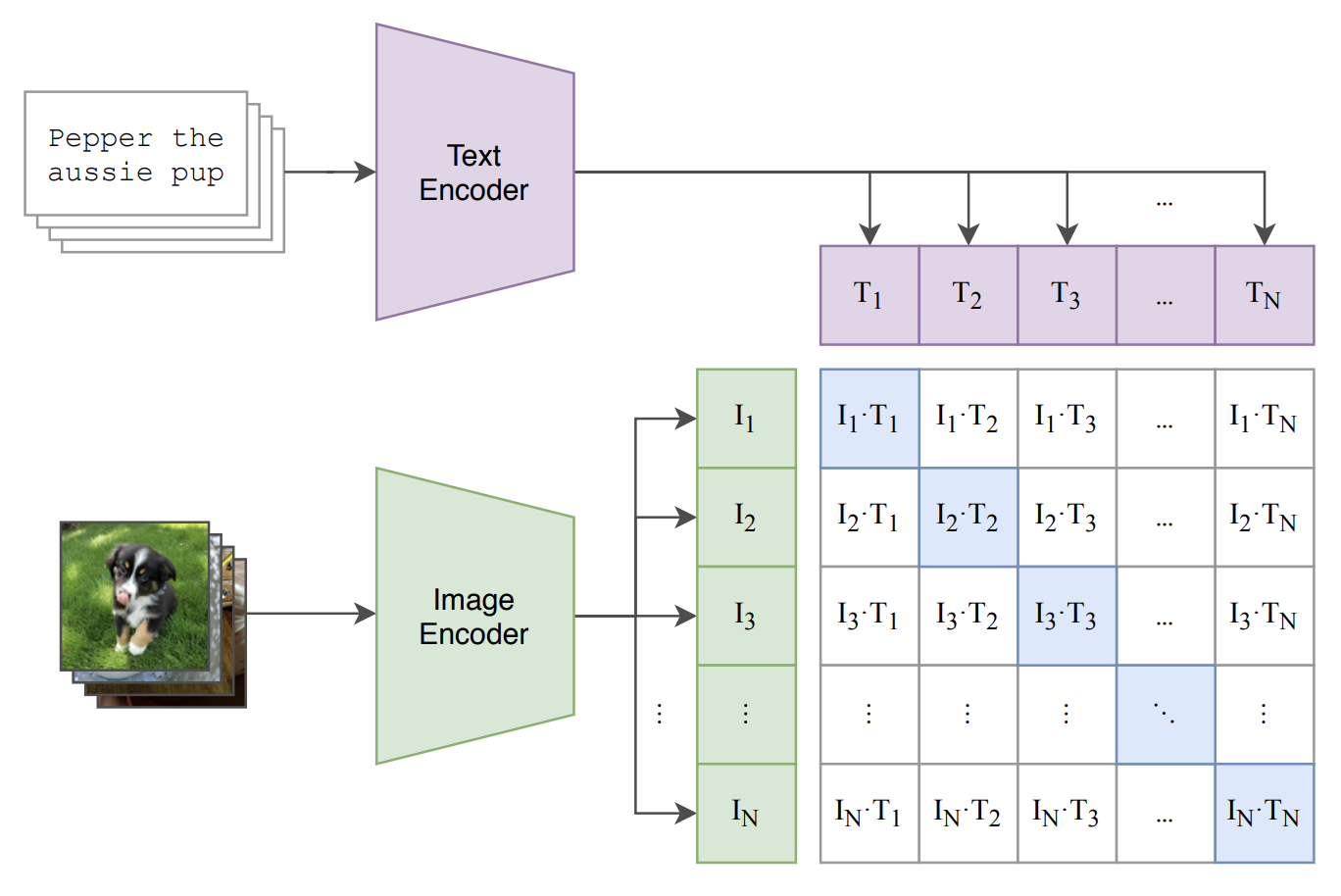
Fig. CLIP Model.
DALLE-2 specifically uses the CLIP model, which was developed by OpenAI in the paper “Learning Transferable Visual Models From Natural Language Supervision”. The CLIP model aims to create a cross-embedding space between text and images. In the figure above, we see the caption “Pepper the aussie pup” accompanied below with its corresponding image. To train a joint-embedding space, the paper took many pairs of pictures together with their captions. The Text Encoder generates the text embedding using Transformers in NLP which is the state of the art for most textual tasks today. The Image Encoder is a separate convolutional network which creates an embedding for our image. With both the text embedding and image embedding we can take the dot product of both representations to obtain the similarity between text and image. The goal of this task is to classify which image belongs to which caption and vice versa. By training the model against this task, we train an embedding space that can both represent images and text. This has powerful applications not only in zero-shot learning (predicting unknown classes of images by using text, etc) but also several down-stream textual/image tasks as we’ve seen with DALLE-2.
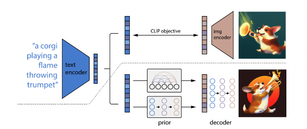
Fig. DALLE-2 Architecture.
The above diagram demonstrates how DALLE-2 is trained with the diffusion and CLIP concepts we’ve described in this article. Above the dotted line is where the training of the CLIP model is done. That is we are learning the joint representation between image and text. Below the dotted line, there are two parts of DALLE-2, the prior and the decoder. The decoder is the reverse diffusion process we’ve described in the previous parts. As we’ve learned from the reverse diffusion process, generating an image requires starting from a noisy image and denoising the image to obtain the generated image. The goal of the prior is to identify parts of the noise distribution and condition the noise on the textual embedding. For example, given the caption “a corgi playing a flame throwing trumpet”, we aim to identify the distribution of noisy images that when passed through the decoder, will generate the corresponding image. The entire network is then jointly trained to allow for conditional generation on the caption.
COLAB Notebook
Feel free to explore the implementation or play around with the modules discussed in this article via our COLAB Notebook.
References
Papers:
- Dhariwal, Prafulla, and Alex Nichol. “Diffusion Models Beat Gans on Image Synthesis.” ArXiv.org, 1 June 2021,
- Ho, Jonathan, et al. “Denoising Diffusion Probabilistic Models.” ArXiv.org, 16 Dec. 2020,
- Luo, Calvin. “Understanding Diffusion Models: A Unified Perspective.” ArXiv.org, 25 Aug. 2022,
- Radford, Alec, et al. “Learning Transferable Visual Models from Natural Language Supervision.” ArXiv.org, 26 Feb. 2021,
Other Articles: