Deep Fake Generation

The use of deep learning methods in deep fake generation has contributed to the rise of fake of fake images which has some very serious ethical dilemmas. We will look at two different ways to generate deepfake pictures and videos, and will then focus in on Image-to-Image Translation. CycleGAN and StarGAN are two different models we will by studying to create deep fake images using Image-to-Image Translation.

Table of Contents

• Introduction
• What is Deepfake
  • Example: Image-to-Image Translation
  • Example: Image Animation
• What is a Generative Adversarial Network (GAN)
• Cycle GAN
  • Motivation
  • Architecture
  • Architecture Blocks and Code Implementation
  • Results
• Star GAN
  • Motivation
  • Architecture
  • Architecture Blocks and Code Implementation
  • Results
• Demo
• References

Introduction

In this post, we will be covering two different models used for image-to-image translation. These models can be used for creating Deepfake media.

What is Deepfake

Deepfake is a term used to describe artificially constructed media that portrays an individual or individuals in a way that suits the creator. For example, creating image to image translations, image animations, audio reconstruction, and more. Deepfakes are created using deep neural networks architectures, such as Generative Adversarial Networks or Autoencoders.

Example: Image-to-Image Translation

Image to image translation is the process of extracting features from a source image and emulating those features in another image. An example would be Neural Style Transfer, where a source image is used to create an art style to transfer to another image.

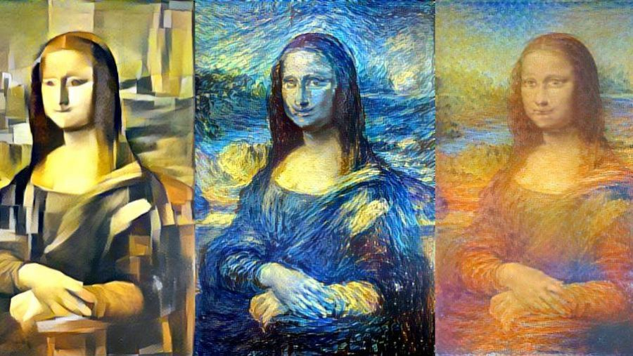
• Fig 1. Example of Neural Style Transfer (Image source: https://www.v7labs.com/blog/neural-style-transfer)

Below are some common architectures seen for image to image translation.

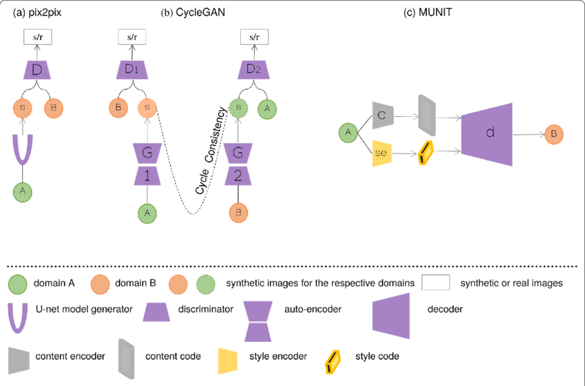
• Fig 2. Example of image to image translation architectures (Image source: https://www.researchgate.net/publication/366191121_Enhancing_cancer_differentiation_with_synthetic_MRI_examinations_via_generative_models_a_systematic_review)

Example: Image Animation

Image Animation is the action of generating a video where the object from an image is animated using the action from a driving video. For example, if we had an image of a water bottle and a driving video of a ball flying across the screen, the output video would be a water bottle flying across the screen. Thus, it will create an animation based on a single image.

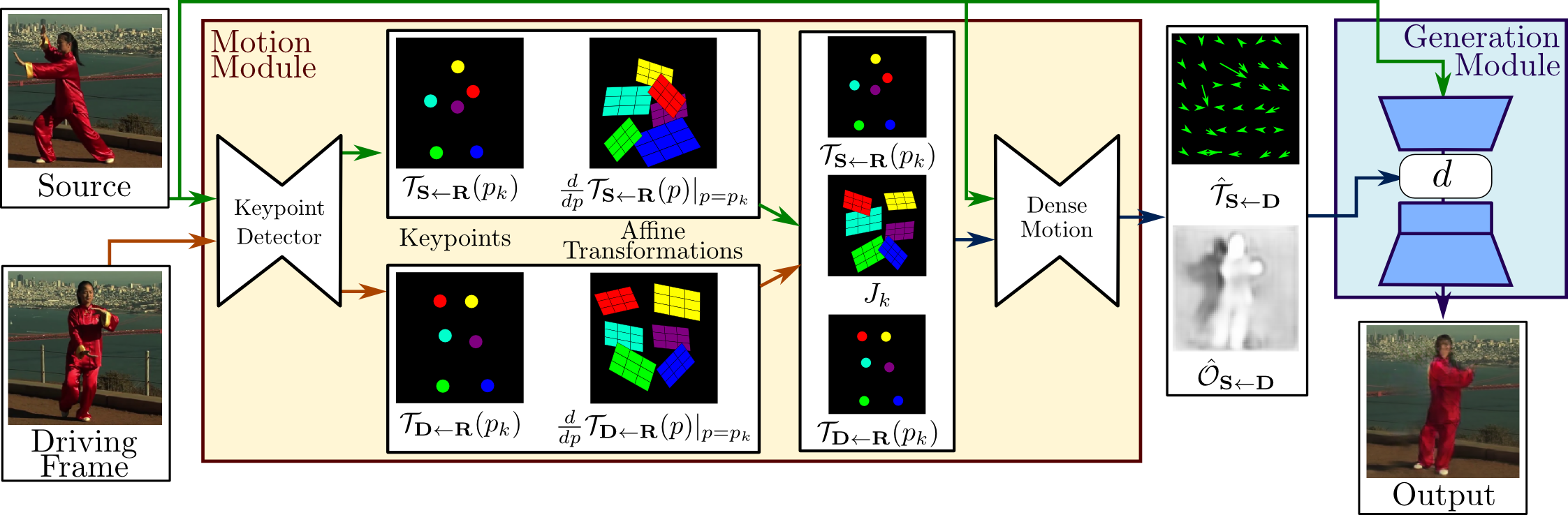
• Fig 3. Example flow of Image Animation (Image Source: [10])

Once applying the model, we would see results similar to the following:

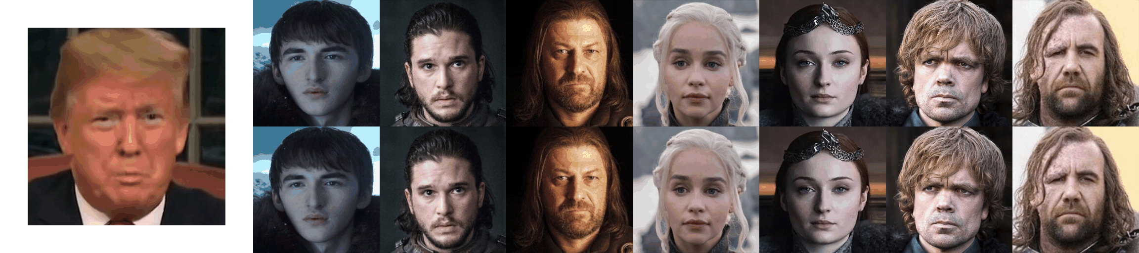
• Figure 4. Example output from Image Animation (Image Source: [9])

What is a Generative Adversarial Network (GAN)

Generative Adversarial Network, or GAN, is the core framework behind a lot of the DeepFake algorithms you may come across. It is an approach to generate a model for a dataset using deep learning priciples. Generative modeling automatically discovers and learns the patterns in the data so that the model can be used to generate new images that could have been a part of the original dataset. GANs train a generative model that consists of two sub-components: the generator models which is trained to generate new images and the discriminator model which tries to classify an image as real or fake. The generative models and the discriminator model are trained together in an adversarial way, meaning until the discrimnator model classifies images incorrectly about half of the time. This would mean that the generator model generates DeepFake images that could pass as being real.

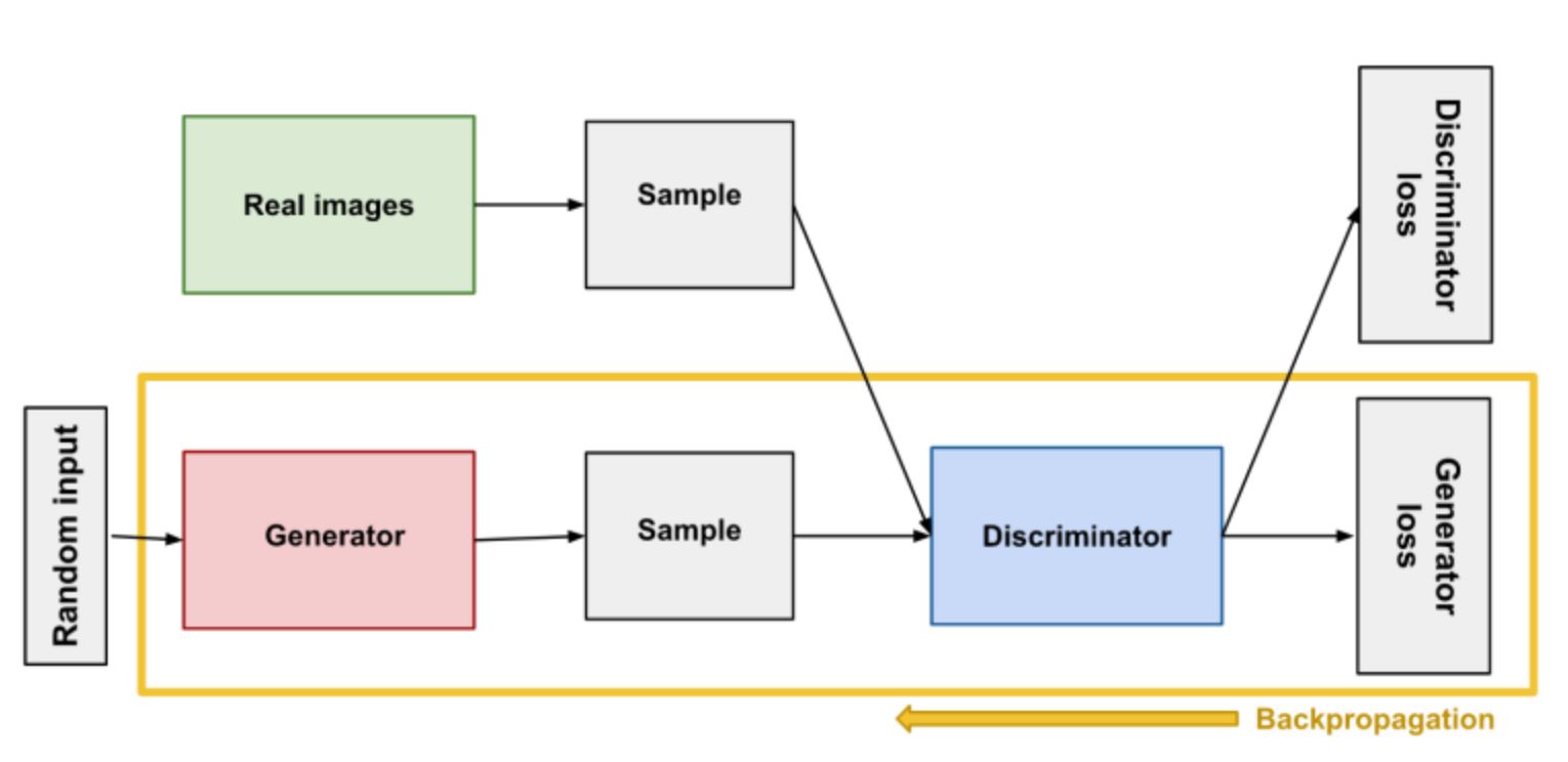
• Fig 5. Example of GAN Flow (Image Source: [11])

Below we look into two different models using ideas from GAN.

Cycle GAN

Motivation

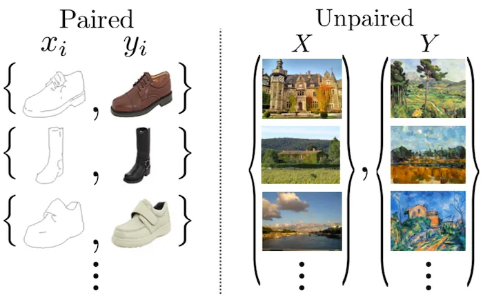
• Fig 6. Example of paired and unpaired images, (Image source: https://towardsdatascience.com/cyclegan-learning-to-translate-images-without-paired-training-data-5b4e93862c8d)

CycleGAN was used in order to use unpaired image to image translations rather than paired image to image translations. This would allow for more training data and more robust outputs for translations. This model seems to work well on tasks that involve color or texture changes, like day-to-night photo translations, or photo-to-painting tasks like collection style transfer. However, tasks that require substantial geometric changes to the image, such as cat-to-dog translations, usually fail [5].

Architecture

The architecture of CycleGAN consists of a generator taken from Johnson et al [3], which consists of 3 convolutional layers, 6 residual block layers, 2 transpose convolutional layers and a final convolution output layer. Should also be noted that all layers similar to Johnson et al are followed by instance normalization.

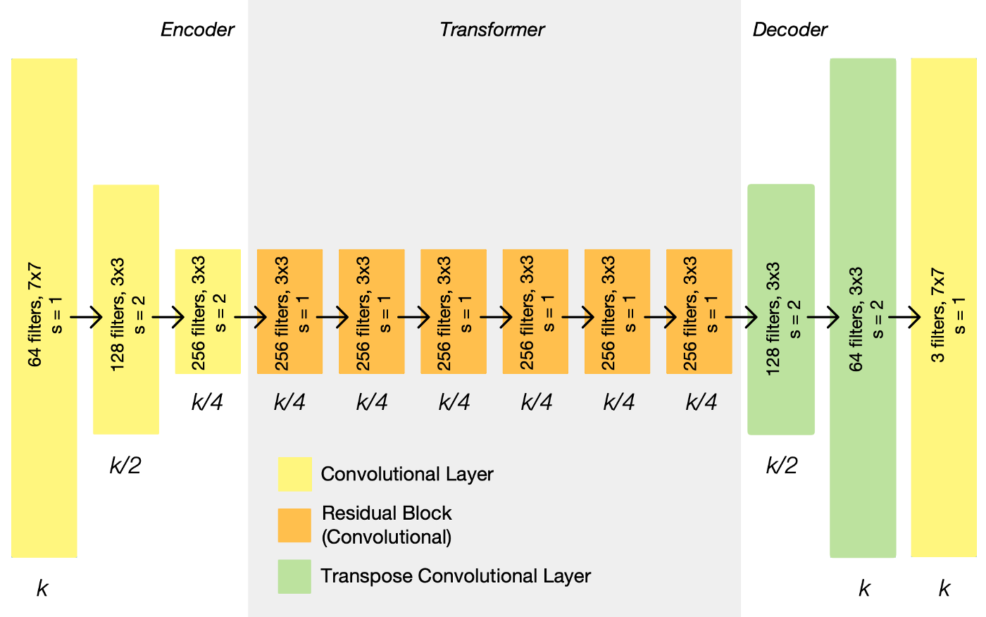
• Fig 7. Example of CycleGAN Generator architecture (Image source: https://towardsdatascience.com/cyclegan-learning-to-translate-images-without-paired-training-data-5b4e93862c8d)

The discriminator uses a 70x70 PatchGAN architecture, which are used to classify 70x70 overlapped images to see if they are real or fake. The PatchGAN architecture consists of 5 convolutional layers with instance normalization [5].

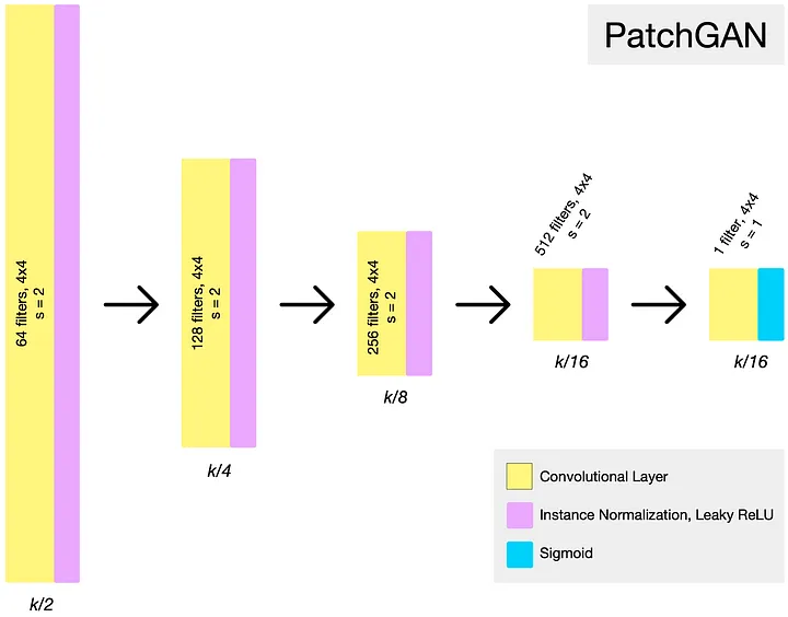
• Fig 8. Example of CycleGAN Discriminator architecture (Image source: https://towardsdatascience.com/cyclegan-learning-to-translate-images-without-paired-training-data-5b4e93862c8d)

The complete model consists of two Generators and two Discriminators. Each Generator/Discriminator pair tries to map an image from one domain to another while the other pair tries to map the reverse of the image.

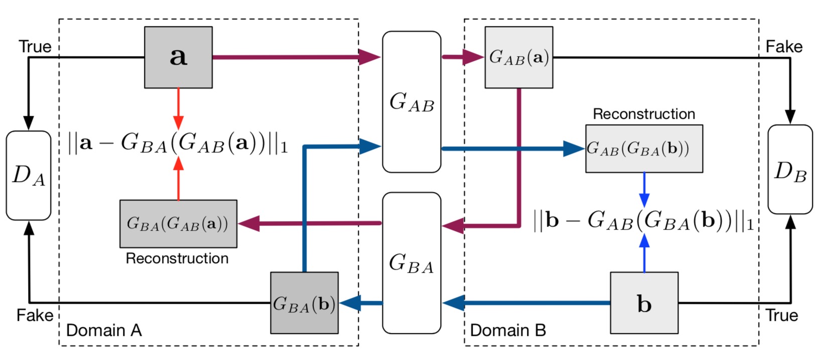
• Fig 9. CycleGAN architecture with all generators and discriminators. (Image source: https://cvnote.ddlee.cc/2019/08/21/image-to-image-translation-pix2pix-cyclegan-unit-bicyclegan-stargan)

Loss Functions

There are two kinds of loss in the CycleGAN architecture. There is the normal adversarial loss that we typically associate with GANs and there is the cyclic loss that is used in the CycleGAN implementation. Since the architecture contains two GAN networks, the mapping functions are from $G : X \to Y$ and $F : Y \to X$ where the discriminators are $D_Y$ and $D_X$ respectively. G will map images from the X domain to the Y domain while $D_Y$ will try to discriminate the images that G mapped. F will do the same thing however, it will do it from the Y domain over to the X domain with $D_X$ trying to discriminate the mapped images.

Log likelihood loss was used for the adversarial loss in Zhu et al’s implementation [7]. The loss function for the adversarial loss is as follows:

This loss function only takes into account the G mapping from X domain to Y domain. In order to optimize loss for the other network, another adversarial loss function would need to be used for the F mapping. So the total loss would need to include two sets of adversarial loss.

Then there is also the cyclic-consistency loss which ensures that $F(G(x)) \approx x$ and $G(F(y)) \approx y$. L1 norm loss was used for the cyclic loss function.

The complete objective function is as follows:

where $\lambda$ controls the importance between the two types of losses.

According to Zhu et al [7], they aim to solve:

Architecture Blocks and Code Implementation

The following code blocks for the CycleGAN implementation were taken from junyanz/pytorch-CycleGAN-and-pix2pix repository.

The code below shows the implementations for creating the CycleGAN model. However, the important thing to note is that the the network architecture is created by calling functions called define_G and define_D which instantiate a generator and discriminator model respectively. The CycleGan model then proceeds to define the optimizers and criterion for the generators and discriminators.

When the CycleGAN model calls the function define_G(), the model accesses the ResnetGenerator class which creates the generator for the CycleGAN model.

class ResnetGenerator(nn.Module):
    """Resnet-based generator that consists of Resnet blocks between a few downsampling/upsampling operations.
    We adapt Torch code and idea from Justin Johnson's neural style transfer project(https://github.com/jcjohnson/fast-neural-style)
    """

    def __init__(self, input_nc, output_nc, ngf=64, norm_layer=nn.BatchNorm2d, use_dropout=False, n_blocks=6, padding_type='reflect'):
        """Construct a Resnet-based generator
        Parameters:
            input_nc (int)      -- the number of channels in input images
            output_nc (int)     -- the number of channels in output images
            ngf (int)           -- the number of filters in the last conv layer
            norm_layer          -- normalization layer
            use_dropout (bool)  -- if use dropout layers
            n_blocks (int)      -- the number of ResNet blocks
            padding_type (str)  -- the name of padding layer in conv layers: reflect | replicate | zero
        """
        assert(n_blocks >= 0)
        super(ResnetGenerator, self).__init__()
        if type(norm_layer) == functools.partial:
            use_bias = norm_layer.func == nn.InstanceNorm2d
        else:
            use_bias = norm_layer == nn.InstanceNorm2d

        model = [nn.ReflectionPad2d(3),
                 nn.Conv2d(input_nc, ngf, kernel_size=7, padding=0, bias=use_bias),
                 norm_layer(ngf),
                 nn.ReLU(True)]

        n_downsampling = 2
        for i in range(n_downsampling):  # add downsampling layers
            mult = 2 ** i
            model += [nn.Conv2d(ngf * mult, ngf * mult * 2, kernel_size=3, stride=2, padding=1, bias=use_bias),
                      norm_layer(ngf * mult * 2),
                      nn.ReLU(True)]

        mult = 2 ** n_downsampling
        for i in range(n_blocks):       # add ResNet blocks

            model += [ResnetBlock(ngf * mult, padding_type=padding_type, norm_layer=norm_layer, use_dropout=use_dropout, use_bias=use_bias)]

        for i in range(n_downsampling):  # add upsampling layers
            mult = 2 ** (n_downsampling - i)
            model += [nn.ConvTranspose2d(ngf * mult, int(ngf * mult / 2),
                                         kernel_size=3, stride=2,
                                         padding=1, output_padding=1,
                                         bias=use_bias),
                      norm_layer(int(ngf * mult / 2)),
                      nn.ReLU(True)]
        model += [nn.ReflectionPad2d(3)]
        model += [nn.Conv2d(ngf, output_nc, kernel_size=7, padding=0)]
        model += [nn.Tanh()]

        self.model = nn.Sequential(*model)

    def forward(self, input):
        """Standard forward"""
        return self.model(input)

This is an implementation of the ResnetBlocks used in the ResnetGenerator model. Which just consists of a convolutional layer, a normalization layer and a ReLU activation layer.

class ResnetBlock(nn.Module):
    """Define a Resnet block"""

    def __init__(self, dim, padding_type, norm_layer, use_dropout, use_bias):
        """Initialize the Resnet block
        A resnet block is a conv block with skip connections
        We construct a conv block with build_conv_block function,
        and implement skip connections in <forward> function.
        Original Resnet paper: https://arxiv.org/pdf/1512.03385.pdf
        """
        super(ResnetBlock, self).__init__()
        self.conv_block = self.build_conv_block(dim, padding_type, norm_layer, use_dropout, use_bias)

    def build_conv_block(self, dim, padding_type, norm_layer, use_dropout, use_bias):
        """Construct a convolutional block.
        Parameters:
            dim (int)           -- the number of channels in the conv layer.
            padding_type (str)  -- the name of padding layer: reflect | replicate | zero
            norm_layer          -- normalization layer
            use_dropout (bool)  -- if use dropout layers.
            use_bias (bool)     -- if the conv layer uses bias or not
        Returns a conv block (with a conv layer, a normalization layer, and a non-linearity layer (ReLU))
        """
        conv_block = []
        p = 0
        if padding_type == 'reflect':
            conv_block += [nn.ReflectionPad2d(1)]
        elif padding_type == 'replicate':
            conv_block += [nn.ReplicationPad2d(1)]
        elif padding_type == 'zero':
            p = 1
        else:
            raise NotImplementedError('padding [%s] is not implemented' % padding_type)

        conv_block += [nn.Conv2d(dim, dim, kernel_size=3, padding=p, bias=use_bias), norm_layer(dim), nn.ReLU(True)]
        if use_dropout:
            conv_block += [nn.Dropout(0.5)]

        p = 0
        if padding_type == 'reflect':
            conv_block += [nn.ReflectionPad2d(1)]
        elif padding_type == 'replicate':
            conv_block += [nn.ReplicationPad2d(1)]
        elif padding_type == 'zero':
            p = 1
        else:
            raise NotImplementedError('padding [%s] is not implemented' % padding_type)
        conv_block += [nn.Conv2d(dim, dim, kernel_size=3, padding=p, bias=use_bias), norm_layer(dim)]

        return nn.Sequential(*conv_block)

    def forward(self, x):
        """Forward function (with skip connections)"""
        out = x + self.conv_block(x)  # add skip connections
        return out

The discriminator model used for the CycleGAN is a PatchGAN implementation. The define_D function in the CycleGAN model accesses this class and creates a PatchGAN.

class NLayerDiscriminator(nn.Module):
    """Defines a PatchGAN discriminator"""

    def __init__(self, input_nc, ndf=64, n_layers=3, norm_layer=nn.BatchNorm2d):
        """Construct a PatchGAN discriminator
        Parameters:
            input_nc (int)  -- the number of channels in input images
            ndf (int)       -- the number of filters in the last conv layer
            n_layers (int)  -- the number of conv layers in the discriminator
            norm_layer      -- normalization layer
        """
        super(NLayerDiscriminator, self).__init__()
        if type(norm_layer) == functools.partial:  # no need to use bias as BatchNorm2d has affine parameters
            use_bias = norm_layer.func == nn.InstanceNorm2d
        else:
            use_bias = norm_layer == nn.InstanceNorm2d

        kw = 4
        padw = 1
        sequence = [nn.Conv2d(input_nc, ndf, kernel_size=kw, stride=2, padding=padw), nn.LeakyReLU(0.2, True)]
        nf_mult = 1
        nf_mult_prev = 1
        for n in range(1, n_layers):  # gradually increase the number of filters
            nf_mult_prev = nf_mult
            nf_mult = min(2 ** n, 8)
            sequence += [
                nn.Conv2d(ndf * nf_mult_prev, ndf * nf_mult, kernel_size=kw, stride=2, padding=padw, bias=use_bias),
                norm_layer(ndf * nf_mult),
                nn.LeakyReLU(0.2, True)
            ]

        nf_mult_prev = nf_mult
        nf_mult = min(2 ** n_layers, 8)
        sequence += [
            nn.Conv2d(ndf * nf_mult_prev, ndf * nf_mult, kernel_size=kw, stride=1, padding=padw, bias=use_bias),
            norm_layer(ndf * nf_mult),
            nn.LeakyReLU(0.2, True)
        ]

        sequence += [nn.Conv2d(ndf * nf_mult, 1, kernel_size=kw, stride=1, padding=padw)]  # output 1 channel prediction map
        self.model = nn.Sequential(*sequence)

    def forward(self, input):
        """Standard forward."""
        return self.model(input)

Results

Using the pretrained models monet2photo and style_monet from the cycleGAN repository, I was able to get the following results:

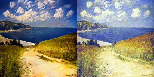
• Fig 10. Monet painting being converted to realistic photo. Original image on right and generated image on left.

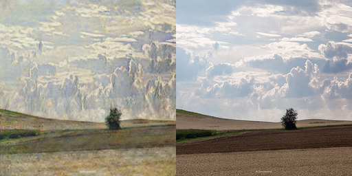
• Fig 11. Realistic photo being converted to monet styled painting. Original image on right and generated image on left.

Dicsussion

With this GAN architecture, it is able to perform better than other GAN architectures primarily because the cycle consistency loss keeps the model stable. The model has to be able to return back to the original image when ran through the other network, so with this it keeps the mappings consistent with each other. It should also be noted that when the models were trained without GAN + forward cycle loss or GAN + backward cycle loss it resulted in training instability and mode collapse, primarily for the removed direction, ensued.

The pretrained models are trained with $\lambda = 10$ for the cycle-consistency loss. The batch sized used is 1 and the learning rate is 0.0002 for the first 100 epochs and linearly decreases rate to zero over the next 100 epochs.

However, there are also images that do not work well with the models. If the image needs to be changed drastically or the images are far to different from the training data provided then the results aren’t as great. For example, on the task of dog→cat transfiguration, the learned translation degenerates into making minimal changes to the input. According to Zhu et al., the failure could be caused by the generator architecture which are designed for more appearance changes rather than geometric transformations. Another factor would be the training data used, for example, using wild horse and zebra images for training so an image containing a human riding a horse would skew the results.

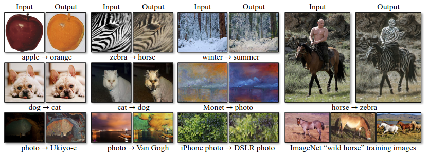
• Fig 12. Table of images that failed the image translation. (Image source: [7])

Star GAN v2

Motivation

StarGAN is a generative adversarial network that learns the mappings among multiple domains using only a single generator and a discriminator, training effectively from images of all domains (Choi 2). The topology could be represented as a star where multi-domains are connected, thus receiveing the name StarGAN. In this article, we will be looking at StarGAN v2. The main differentiation between versions is that v2 is “a scalable approach that can generate diverse images across multiple domains” (Choi v2 pg2). The domain label is replaced with the domain specific style code. The goal is that v2 will yield better results in terms of visual qulaity and diveristy than the original StarGAN.

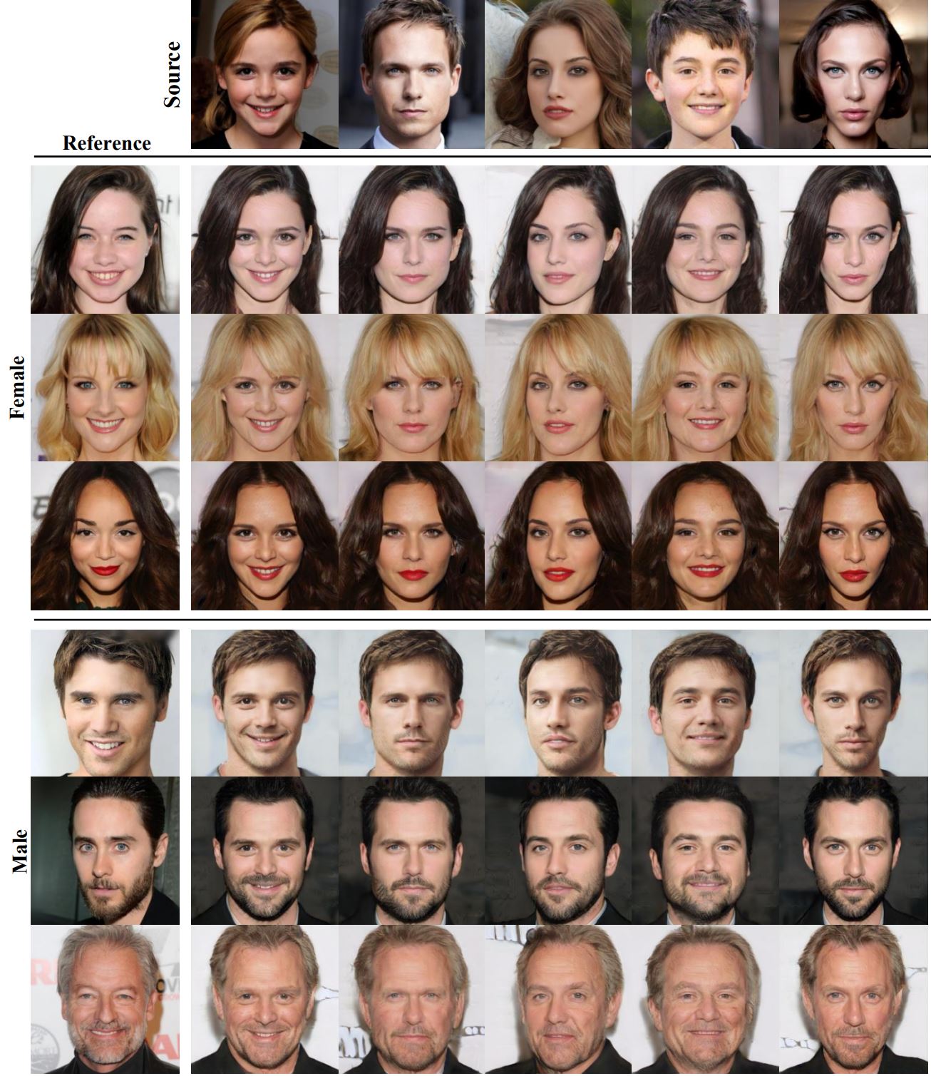
• Fig 13. Example of image synthesis results on CelebA dataset using StarGAN v2. The source and reference images are in the first rown and column, and they are real images, while the rest of the images are generated. (Image source: [6])

StarGAN consists of two modules, a discriminator and a generator. The discriminator learns to differentiate between real and fake images and begins to clssify the real images with its proper domain. The generator takes an image and a target domain label as input and generates a fake image with them. The target domain label is then spatially replicated and concatenated with the image given as input. The generator attempts to reconstruct the orginal image via the fake image when given the original domain label. Lastly, the generator tries to generate images that are almost identical to the real images and will be classified as being from the target domain by the discriminator.

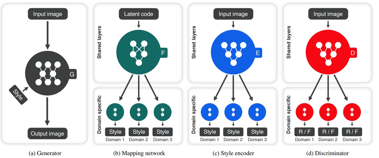
• Fig 14. Example flow of StarGAN v2 where D represents the discriminator, G represents the generator, F represents the mapping network, and E represents the style encoder (Image Source: [6])

The overarching goal of StarGAN v2 is to train a generator that can generate diverse images of each of the domains that correspond to an image. A domain specific style vectors in the learned style space of each of the trains and then train the generator to reflect the style vectors.

Architecture

The Generator Architecture consists of 4 downsampling blocks that use instance normalization (IN), four intermediate blocks, and four upsampling blocks that use adaptive instance normalization (AdaIN). These blocks all have pre-activation residual units. Style code is injected into all the AdaIN layers.

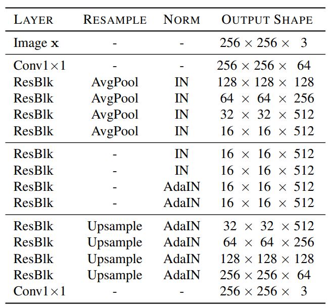
• Fig 15. Example of StarGAN v2 Generator Architecture (Image source: [6])

The Mapping Network Architecture consists of an MLP with k (number of domains) output branches. Four fully connected layers are shared among domains, and they are followed by four fully conected layers for each individual domain.

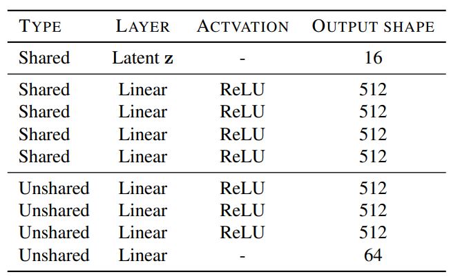
• Fig 16. Example of StarGAN v2 mapping netwrok architecture (Image source: [6])

The Style Encoder Architecture consists of CNN with k (number of domains) output branches. Six pre-activation residual blocks are shared among domains, and they are followed by one fully connected layer for each individual domain.

The Discriminator Architecture consists of six pre-activation residual blocks with leaky ReLY. k (number of domains) fully connected layers are used for real/fake classification among each domain.

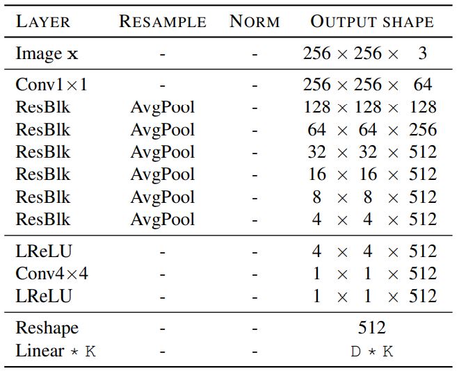
• Fig 17. Example of StarGAN v2 style encoder and discriminator architecture, where D and K are the output dimensions (Image Source: [6])

Loss Functions

The StarGAN v2 netwrok is trained using adversarial objective, style reconstruction, style diversification, and preserving source characteristics. (Equation Source: [6])

• Adversarial Objective:

  The generator G takes an image x and $\tilde{s}$ as input and learns to generate an output image G(x, $\tilde{s}$ ) via adversarial loss which is defined as

where x represents the latent code, $\tilde{y}$ represents the target domain, $\tilde{s}$ represents the target style code

• Style Reconstruction:

  To ensure the generator utillzes the style code, $\tilde{s}$, when generating G(x, $\tilde{s}$), we need to use style reconstruction loss which is defined as

• Style Diversification:

  To enable the generator to produce diverse images, the generator is regularized with diversity sensitive loss which is defined as

where $\tilde{s_1}$ and $\tilde{s_2}$ are produced by F conditioned on two random latent codes $z_{1}$ and $z_{2}$

• Preserving Source Characteristics:

  To ensure the generated image G(x, $\tilde{s}$) preserves the domain invariant characteristics, we need to use cycle consitency loss which is defined as

where $\hat{s}$ = $E_{y}(x)$ is the estimated style code of the input image x

• Full Objective:

  The full object is defined as

where $\lambda_{sty}$, $\lambda_{ds}$, and $\lambda_{cyc}$ are hyperparameters for each term

Architecture Blocks and Code Implementation

The code for the part of the init() and the follow() functions for the Generator is as follows.

class Generator(nn.Module):
    def __init__(self, img_size=256, style_dim=64, max_conv_dim=512, w_hpf=1):
        super().__init__()
        dim_in = 2**14 // img_size
        self.img_size = img_size
        self.from_rgb = nn.Conv2d(3, dim_in, 3, 1, 1)
        self.encode = nn.ModuleList()
        self.decode = nn.ModuleList()
        self.to_rgb = nn.Sequential(
            nn.InstanceNorm2d(dim_in, affine=True),
            nn.LeakyReLU(0.2),
            nn.Conv2d(dim_in, 3, 1, 1, 0))

        ...

    def forward(self, x, s, masks=None):
        x = self.from_rgb(x)
        cache = {}
        for block in self.encode:
            if (masks is not None) and (x.size(2) in [32, 64, 128]):
                cache[x.size(2)] = x
            x = block(x)
        for block in self.decode:
            x = block(x, s)
            if (masks is not None) and (x.size(2) in [32, 64, 128]):
                mask = masks[0] if x.size(2) in [32] else masks[1]
                mask = F.interpolate(mask, size=x.size(2), mode='bilinear')
                x = x + self.hpf(mask * cache[x.size(2)])
        return self.to_rgb(x)

The code for the Discriminator is as follows.

class Discriminator(nn.Module):
    def __init__(self, img_size=256, num_domains=2, max_conv_dim=512):
        super().__init__()
        dim_in = 2**14 // img_size
        blocks = []
        blocks += [nn.Conv2d(3, dim_in, 3, 1, 1)]

        repeat_num = int(np.log2(img_size)) - 2
        for _ in range(repeat_num):
            dim_out = min(dim_in*2, max_conv_dim)
            blocks += [ResBlk(dim_in, dim_out, downsample=True)]
            dim_in = dim_out

        blocks += [nn.LeakyReLU(0.2)]
        blocks += [nn.Conv2d(dim_out, dim_out, 4, 1, 0)]
        blocks += [nn.LeakyReLU(0.2)]
        blocks += [nn.Conv2d(dim_out, num_domains, 1, 1, 0)]
        self.main = nn.Sequential(*blocks)

    def forward(self, x, y):
        out = self.main(x)
        out = out.view(out.size(0), -1)  # (batch, num_domains)
        idx = torch.LongTensor(range(y.size(0))).to(y.device)
        out = out[idx, y]  # (batch)
        return out

The code for the style encoder is as follows.

class StyleEncoder(nn.Module):
    def __init__(self, img_size=256, style_dim=64, num_domains=2, max_conv_dim=512):
        super().__init__()
        dim_in = 2**14 // img_size
        blocks = []
        blocks += [nn.Conv2d(3, dim_in, 3, 1, 1)]

        repeat_num = int(np.log2(img_size)) - 2
        for _ in range(repeat_num):
            dim_out = min(dim_in*2, max_conv_dim)
            blocks += [ResBlk(dim_in, dim_out, downsample=True)]
            dim_in = dim_out

        blocks += [nn.LeakyReLU(0.2)]
        blocks += [nn.Conv2d(dim_out, dim_out, 4, 1, 0)]
        blocks += [nn.LeakyReLU(0.2)]
        self.shared = nn.Sequential(*blocks)

        self.unshared = nn.ModuleList()
        for _ in range(num_domains):
            self.unshared += [nn.Linear(dim_out, style_dim)]

    def forward(self, x, y):
        h = self.shared(x)
        h = h.view(h.size(0), -1)
        out = []
        for layer in self.unshared:
            out += [layer(h)]
        out = torch.stack(out, dim=1)  # (batch, num_domains, style_dim)
        idx = torch.LongTensor(range(y.size(0))).to(y.device)
        s = out[idx, y]  # (batch, style_dim)
        return s

Results

Here are the results from running the trained model with different learning rates, weight decays, alpha, and beta values.

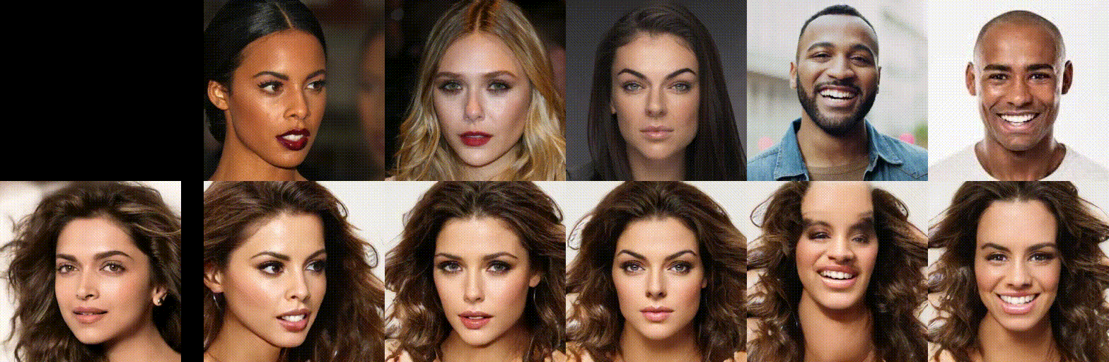
• Fig 18. Chosen Model: lr=1e-4, fLr=1e-6, alpha=0, beta=0.99, weightDecay=1e-4

• Fig 19. Alternate Model 1: lr=1e-4, fLr=1e-6, alpha=.5, beta=0.5, weightDecay=1e-4

• Fig 20. Alternate Model 2: lr=1e-4, fLr=1e-6, alpha=.5, beta=0.5, weightDecay=1e-5

• Fig 21. Alternate Model 3: lr=1e-4, fLr=1e-6, alpha=.5, beta=0.5, weightDecay=1e-3

Running the model on different images with the best model, the one listed in Fig 17 results in the following:

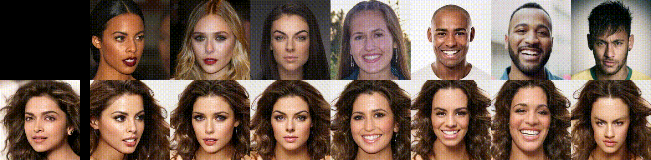
• Fig 22. Chosen Model with cropped images

Dicsussion

As we can see from the results, this model heavily relies on images being cropped similarly to the data used to train the model. For example, we can see that the image with the guy in the blue shirt is not generated correctly in some instances. We can specifically see this in the eyebrows and neck area. However, when we look at all three women, who were in the train dataset, their generations look perfect.

You can see that the hairstyle, makeup, and more from the reference image is applied to the facial expression of the source image.

One downside of this method is hair generation. You can see in the first source image that generating some of the women’s hairstyles had some small issue. This is also the case when generating the hair on the source images on the right hand side. Facial hair also proves to be an issue in this model. When looking at the guy in the blue shirt, the deepfake generation images still have pieces leftover from the beard. However, it is not the full beard that we can see in the source image. This can be attributed to a training dataset that is lacking in men with beards. I think the model would be better if the source image’s facial hair was removed in the final deepfake generation image.

The model with lr-1e-4, fixed lr = 1e-6, alhpa=0, beta = .99, and weightDecay = 1e-4 is the best because of the generation of featuers. The hairstyles are slightly better in this model (Fig 17). The flyaways and leftover remnants from the source image are not as apparent in the chosen model than the other ones. The final resulting colors are also slighly better in the chosen model. The shape of the lips is also slightly better in the chosen model. We wanted the shape to be the same as the source image, and that is the case in the chosen model. The eye shape is also better. This is apparent in the first source image. You can see that the eye shape in the generated image matches the eye shap ein the source image perfect. It is not affacted by the reference image at all, which is the goal. The color of the eyes and makeup, however, are modified to match the reference image, which is what we want.

There are multiple reasons why StyleGAN v2 is superior to other deep fake image generation models. Because the style code is separately generated per domain and style encoder, the generator can only focus on using the style code, whose information from the domain can be found using the mapping network. Additionally, the model is able to render many distinctive styles, such as bangs, beard, makeup, and hairstyle. In other models, only the color distribution of reference images are matched. StyleGAN v2 also produces high quality images across all domains, while other models do not. Because other models are trained for each pair of domains, the output quality will differ across the different domains.

Some of the biggest changes to StyleGAN v2 include weight demodulation, lazy regularization, path length regularization, progressive growth, and large networks. These changes resulted in StyleGAN v2 being superior to StyleGAN. For example, the style space is produced by learned transformations in v2, providing it more flexibility. This resulted in better generated images that could be mistaken for real images. StyleGAN also has blob-life artifacts in the generated image, making it harder for a person to beleive it was not generated. This stems from using instance normalization in AdaIN, which was targeted for style transfer to replace the style in one image with one in the other. This issue is not apparent in StyleGAN v2 and seen in the generated result images.

I believe the factor that had the biggest impact on the results being better than StyleGAN was the weight demodulation. It removed how the constant was processed at the beginning of training, made it so that the mean was not needed when normalizing the different features, and moved the noise module outside the style module. Because of these changes, the blob-like features were not apparent in the StyleGAN v2 generated images. And as stated previously, this was the biggest issue with StyleGAN. Because this issue was resolved, we see much better images in StyleGANv2 that would have a greater likelihood of passing for a real image.

I think having a StyleEncoder also made a big difference compared to other image generation techniques. It allowed the style to be translated pretty well in most of the images.

Demo

Click the Picture to Watch the Video!

link to Google Folder: https://drive.google.com/drive/folders/1omGMAXLLt7Bc2HivJ6o-6-96DmPh6OPH?usp=sharing

link to Google Collab: https://colab.research.google.com/drive/1vEm8I2ZddkUOCu0pFBUWhIdxdcnbG_mY?usp=sharing

References

[1] Brownlee, Jason. “A Gentle Introduction to Generative Adversarial Networks (Gans).” MachineLearningMastery.com, 19 July 2019, https://machinelearningmastery.com/what-are-generative-adversarial-networks-gans/.

https://github.com/Deepfakes/

[2] Goodfellow, Ian J., et al. Generative Adversarial Networks. 2014. DOI.org (Datacite), https://doi.org/10.48550/ARXIV.1406.2661.

https://github.com/eriklindernoren/PyTorch-GAN/blob/master/implementations/gan/gan.py

[3] Johnson, Justin, et al. Perceptual Losses for Real-Time Style Transfer and Super-Resolution. arXiv, 26 Mar. 2016. arXiv.org, https://doi.org/10.48550/arXiv.1603.08155.

[4] Tolosana, Ruben, et al. DeepFakes and Beyond: A Survey of Face Manipulation and Fake Detection. 2020. DOI.org (Datacite), https://doi.org/10.48550/ARXIV.2001.00179.

https://github.com/deepfakes/faceswap

[5] Wolf, Sarah. “CycleGAN: Learning to Translate Images (Without Paired Training Data).” Medium, 20 Nov. 2018, https://towardsdatascience.com/cyclegan-learning-to-translate-images-without-paired-training-data-5b4e93862c8d.

[6] Choi, Yunjey, et al. “Stargan v2: Diverse Image Synthesis for Multiple Domains.” ArXiv.org, 26 Apr. 2020, https://arxiv.org/abs/1912.01865.

[7] Zhu, Jun-Yan, et al. Unpaired Image-to-Image Translation Using Cycle-Consistent Adversarial Networks. arXiv, 24 Aug. 2020. arXiv.org, https://doi.org/10.48550/arXiv.1703.10593.

[8] “Pytorch-CycleGAN-and-Pix2pix/Models at Master · Junyanz/Pytorch-CycleGAN-and-Pix2pix.” GitHub, https://github.com/junyanz/pytorch-CycleGAN-and-pix2pix. Accessed 26 Feb. 2023.

[9] Cretin, Nathanael. “[Part 1/2] Using Distributed Learning for Deepfake Detection.” Labelia (Ex Substra Foundation), Labelia (Ex Substra Foundation), 8 Oct. 2021, https://www.labelia.org/en/blog/deepfake1.

[10] Jingles (Jing, Hong). “Realistic Deepfakes in 5 Minutes on Colab.” Medium, Towards Data Science, 27 Nov. 2020, https://towardsdatascience.com/realistic-deepfakes-colab-e13ef7b2bba7.

[11] Mach, Joey. “Deepfakes: The Ugly, and the Good.” Medium, Towards Data Science, 2 Dec. 2019, https://towardsdatascience.com/deepfakes-the-ugly-and-the-good-49115643d8dd.

[12] Hui, Jonathan. “Gan - Stylegan & stylegan2.” Medium, Medium, 10 Mar. 2020, https://jonathan-hui.medium.com/gan-stylegan-stylegan2-479bdf256299.