Text Guided Image Generation
Text-to-image models are machine learning models which take as input a natural language description and produce an image matching the given description. We will explore the architecture and design of one such model, Stable Diffusion, and explore extensions of Stable Diffusion through experiments with prompt-to-prompt editing and model finetuning.
- Introduction
- Stable Diffusion
- Prompt-to-Prompt Editing
- Finetuning
- Societal Impact
- Conclusion
- Code
- References
Video 1. Spotlight Overview.
Introduction
Stable Diffusion is an open-source, state-of-the-art text-to-image model. In this paper, we take an in-depth look at Stable Diffusion itself and extend its applications with Prompt-to-Prompt editing and finetuning. With prompt-to-prompt, we explore the usage of cross-attention maps and how we can leverage them to precisely modify specific parts of a generated image while preserving the rest of the image. For fine-tuning, we finetune Stable Diffusion on a pokemon dataset to create pokemon-like outputs, comparing the before and after results of such finetuning. We conclude with an assessment of the capabilities and limitations of Stable Diffusion, and talk about its potential societal impact.
Stable Diffusion
Stable Diffusion is a latent text-to-image diffusion model. One downside of standard diffusion models is that they work sequentially on the whole image, operating in the pixel space which makes both training and inference times quite significant. To help address this computation problem while maintaining high-quality results, Rombach et. al propose departing from the pixel space and apply these diffusion models in the latent space learned by powerful pre-trained autoencoders.
Image Compression Model
Stable Diffusion’s compression model consists of an autoencoder trained by both perceptual loss and a patch-based adversarial objective. More precisely, given an RGB image \(x\in \mathbb{R}^{H\times W \times 3}\), the encoder \(\mathcal{E}\) encodes \(x\) into a latent representation \(z = \mathcal{E}(x)\), which captures a more fundamental semantic meaning of the image. The decoder D is able to reconstruct the image from the latent, giving \(\tilde{x} = \mathcal{D}(z)= \mathcal{D}(\mathcal{E}(x))\), where \(z \in \mathbb{R}^{h\times w \times c}\). The encoder is thus downsampling the image by a factor \(f = H/h = W/w\).
We can see how the Encoder is implemented with the following code snippets. Take note of the downsampling and then the latent rescaling which is applied after encoding:
class Downsample(nn.Module):
    def __init__(self, in_channels, with_conv):
        super().__init__()
        self.with_conv = with_conv
        if self.with_conv:
            # no asymmetric padding in torch conv, must do it ourselves
            self.conv = torch.nn.Conv2d(in_channels,
                                        in_channels,
                                        kernel_size=3,
                                        stride=2,
                                        padding=0)

    def forward(self, x):
        if self.with_conv:
            pad = (0,1,0,1)
            x = torch.nn.functional.pad(x, pad, mode="constant", value=0)
            x = self.conv(x)
        else:
            x = torch.nn.functional.avg_pool2d(x, kernel_size=2, stride=2)
        return x
class Encoder(nn.Module):
    def forward(self, x):
        # timestep embedding
        temb = None

        # downsampling
        hs = [self.conv_in(x)]
        for i_level in range(self.num_resolutions):
            for i_block in range(self.num_res_blocks):
                h = self.down[i_level].block[i_block](hs[-1], temb)
                if len(self.down[i_level].attn) > 0:
                    h = self.down[i_level].attn[i_block](h)
                hs.append(h)
            if i_level != self.num_resolutions-1:
                hs.append(self.down[i_level].downsample(hs[-1]))

        # middle
        h = hs[-1]
        h = self.mid.block_1(h, temb) # ResnetBlock
        h = self.mid.attn_1(h)
        h = self.mid.block_2(h, temb) # ResnetBlock

        # end
        h = self.norm_out(h) # GroupNorm
        h = nonlinearity(h)
        h = self.conv_out(h)
        return h
class LatentRescaler(nn.Module):
    def __init__(self, factor, in_channels, mid_channels, out_channels, depth=2):
        super().__init__()
        # residual block, interpolate, residual block
        self.factor = factor
        self.conv_in = nn.Conv2d(in_channels,
                                 mid_channels,
                                 kernel_size=3,
                                 stride=1,
                                 padding=1)
        self.res_block1 = nn.ModuleList([ResnetBlock(in_channels=mid_channels,
                                                     out_channels=mid_channels,
                                                     temb_channels=0,
                                                     dropout=0.0) for _ in range(depth)])
        self.attn = AttnBlock(mid_channels)
        self.res_block2 = nn.ModuleList([ResnetBlock(in_channels=mid_channels,
                                                     out_channels=mid_channels,
                                                     temb_channels=0,
                                                     dropout=0.0) for _ in range(depth)])

        self.conv_out = nn.Conv2d(mid_channels,
                                  out_channels,
                                  kernel_size=1,
                                  )

    def forward(self, x):
        x = self.conv_in(x)
        for block in self.res_block1:
            x = block(x, None)
        x = torch.nn.functional.interpolate(x, size=(int(round(x.shape[2]*self.factor)), int(round(x.shape[3]*self.factor))))
        x = self.attn(x)
        for block in self.res_block2:
            x = block(x, None)
        x = self.conv_out(x)
        return x
Latent Diffusion Model
As a high level overview, diffusion models are probabilistic models involving two main steps: a forward diffusion process and a reverse diffusion process. The key idea is to gradually add noise to input samples through a Markov chain of diffusion steps during the forward process and to train a model to learn how to reverse the diffusion process in order to construct realistic images from noise. These models can be interpreted as an equally weighted sequence of denoising autoencoders \(\epsilon_\theta(x_t, t); t = 1 . . . T\), which are trained to predict a denoised variant of their input \(x_t\), where \(x_t\) is a noisy version of the input \(x\). The corresponding objective for diffusion models can be simplified as
\[L := \mathbb{E}_{x,\epsilon\sim \mathcal{N}(0,1),t}\left[\| \epsilon - \epsilon_\theta(x_t, t)\|^2_2 \right]\]Here is a helpful graphical model depicting the diffusion process:
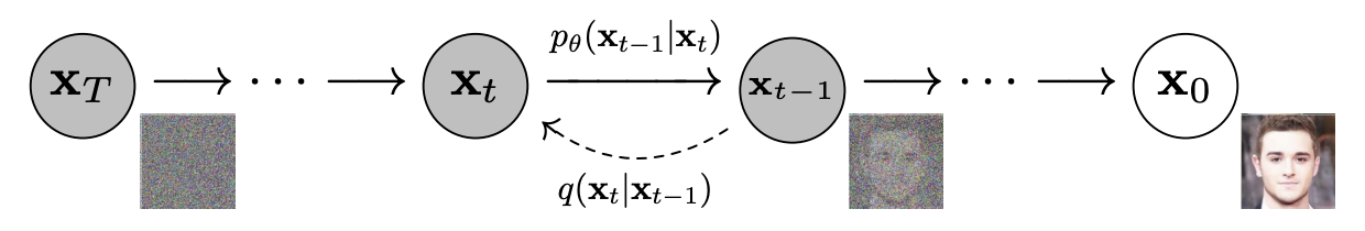 Fig 1: Diffusion Process [2].
Stable Diffusion takes the latent representations generated by the VAE encoder and applies this diffusion process, rewriting the objective as
\[L := \mathbb{E}_{\mathcal{E}(x),\epsilon\sim \mathcal{N}(0,1),t}\left[\| \epsilon - \epsilon_\theta(z_t, t)\|^2_2 \right]\]Using a UNet backbone, the model is then able to efficiently denoise samples from the distribution \(p(z)\) to obtain latent representations of the image. Then, this can be efficiently decoded back to the pixel space using a single pass through the decoder D. The denoising step can also be optionally conditioned on text or images via a cross-attention mechanism. For conditioning on text, the pretrained CLIP ViT-L/14 text encoder is used to transform text prompts to an embedding space. Figure 2 depicts this architecture well for us.
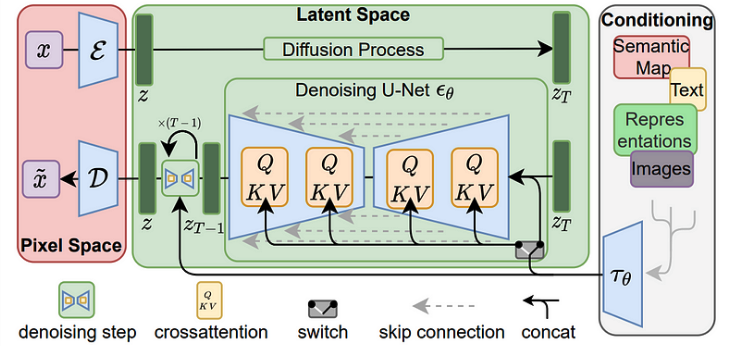 Fig 2: Latent Diffusion Architecture. Image from the paper.
Conditioning Mechanism
Like other generative models, Stable Diffusion can model conditional distributions of the form \(p(z|y)\) with a conditional denoising autoencoder \(\epsilon_\theta(z_t, t, y)\). By augmenting the underlying UNet backbone of Diffusion Models with the cross-attention mechanism, Stable Diffusion is able to be a more flexible conditional image generator. To pre-process \(y\), a domain specific encoder \(\tau_\theta\) projects \(y\) to an intermediate representation \(\tau_\theta(y)\in \mathbb{R}^{M\times d_\tau}\), which is then mapped to the intermediate layers of UNet via a cross-attention layer implementing \(\textrm{Attention}(Q,K,V)=\textrm{softmax}\left(\frac{QK^T}{\sqrt d}\right)\). Finally, based on image-conditioning pairs, the conditional Latent Diffusion Model is learned via
\[L := \mathbb{E}_{\mathcal{E}(x),y,\epsilon\sim \mathcal{N}(0,1),t}\left[\| \epsilon - \epsilon_\theta(z_t, t, \tau_\theta(y))\|^2_2 \right]\]Performance
Stable Diffusion outperforms prior diffusion based approaches on all but the LSUN_Bedrooms dataset, despite using roughly half the parameters and requiring 4-times less training resources.
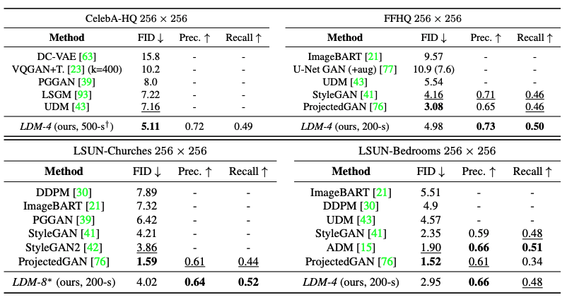 Table 1: Evaluation metrics for unconditional image synthesis [1].
Table 2: Evaluation metrics for text-conditional image synthesis on the \(256 \times 256\)-sized MS-COCO dataset [1].
Additionally, Latent Diffusion Models consistently improves upon GAN-based methods in Precision and Recall, suggesting the advantages of likelihood-based training objectives over adversarial approaches.
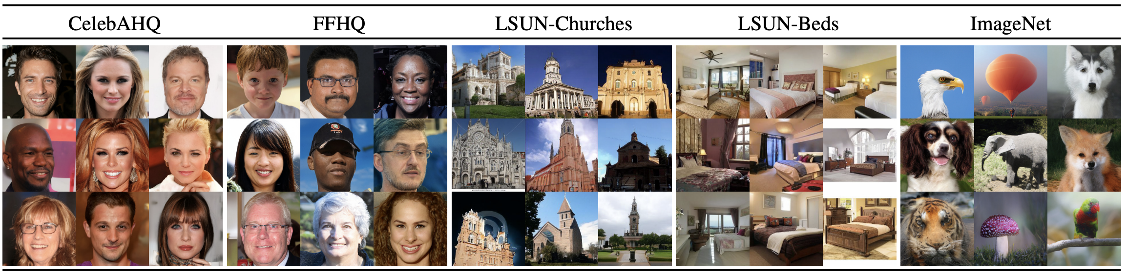 Figure 3: \(256 \times 256\) Samples from LDMs.
With the use of the latent space, Stable Diffusion significantly reduces computational requirements compared to pixel-based approaches while still achieving impressive image quality. However, because sampling is done sequentially, the sampling process remains slower than that of GANs. Furthermore, when high precision is required, the usage of LDMs can be questioned. Although loss of image quality is small, their reconstruction capability can become a bottleneck for tasks requiring fine-grained accuracy in the pixel space.
Prompt-to-Prompt Editing
To take a closer look at the capabilities and limitations of Stable Diffusion, we explored Prompt-To-Prompt image editing via cross-attention control. By controlling the cross-attention maps, we can see the correlation between pixels in the image and words in the prompt. We must use the cross-attention layers because they control how the spatial layout of the image relates to each word in the prompt.
If we were to modify text prompts on Stable Diffusion without cross-attention control, the generated image would be completely different. With prompt-to-prompt editing, we can specifically target and modify only portions of the image, while preserving the rest. We explore various areas of image refinement such as replacement edit, prompt refinement, and attention re-weighting on the final outputted image. The diagram below shows the cross-attention maps in the text-to-image process as well as how each process affects the cross-attention maps:
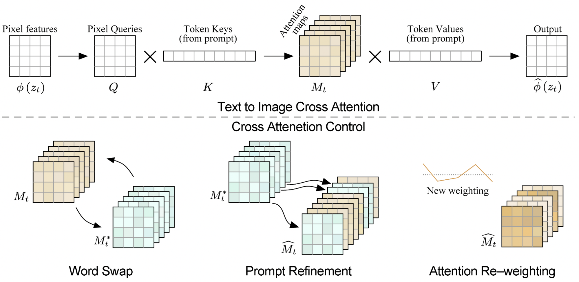 Fig 4: Cross Attention Control.
The corresponding code for registering attention control can be seen here:
def forward(x, context=None, mask=None):
    batch_size, sequence_length, dim = x.shape
    h = self.heads
    q = self.to_q(x)
    is_cross = context is not None
    context = context if is_cross else x
    k = self.to_k(context)
    v = self.to_v(context)
    q = self.reshape_heads_to_batch_dim(q)
    k = self.reshape_heads_to_batch_dim(k)
    v = self.reshape_heads_to_batch_dim(v)

    sim = torch.einsum("b i d, b j d -> b i j", q, k) * self.scale

    if mask is not None:
        mask = mask.reshape(batch_size, -1)
        max_neg_value = -torch.finfo(sim.dtype).max
        mask = mask[:, None, :].repeat(h, 1, 1)
        sim.masked_fill_(~mask, max_neg_value)

    # attention, what we cannot get enough of
    attn = sim.softmax(dim=-1)
    attn = controller(attn, is_cross, place_in_unet)
    out = torch.einsum("b i j, b j d -> b i d", attn, v)
    out = self.reshape_batch_dim_to_heads(out)
    return to_out(out)
https://github.com/google/prompt-to-prompt/blob/main/ptp_utils.py
Cross Attention Visualization
By visualizing cross-attention maps, we can see more clearly how each word in the prompt influences each pixel in the final image. For example, in Figure 5, we can see that the word “rat” directly affects the pixels where the rat is drawn while not affecting the other areas of the image as much. The same can be seen with the word “apartment” where it affects the background of the image more, as we expect.
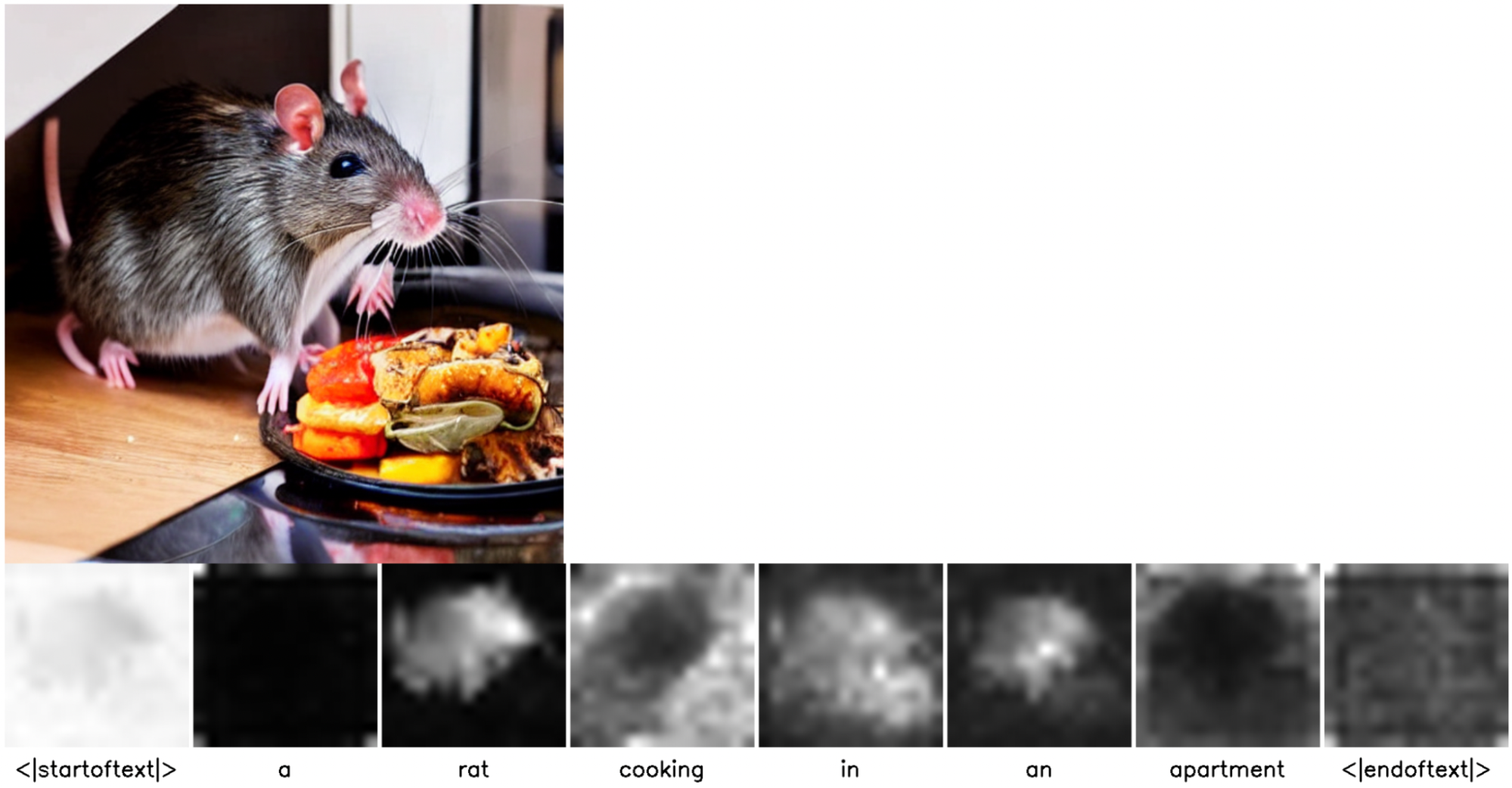 Fig 5: Cross Attention Maps for the prompt “A rat cooking in an apartment”.
Replacement Editing
Knowing these cross-attention maps, we further experiment with word replacement editing. This is when we replace exactly one word in the prompt while keeping all other words the same in order to edit one specific area of the image. For instance, we ran the original prompt “A rat cooking in an apartment” and changed the word “rat” to “dog” to get the final prompt “A dog cooking in an apartment”.The results for this edit without prompt-to-prompt and with prompt-to-prompt are shown in Figures 6 and 7, respectively.
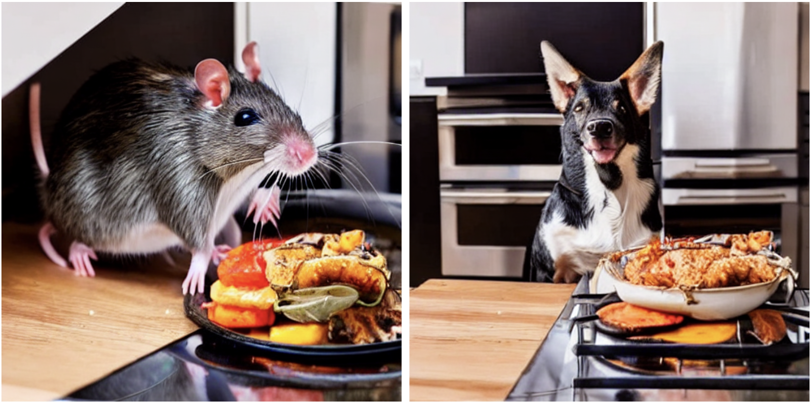 Fig 6: Editing text from “A rat cooking in an apartment” to “A dog cooking in an apartment” without prompt-to-prompt.
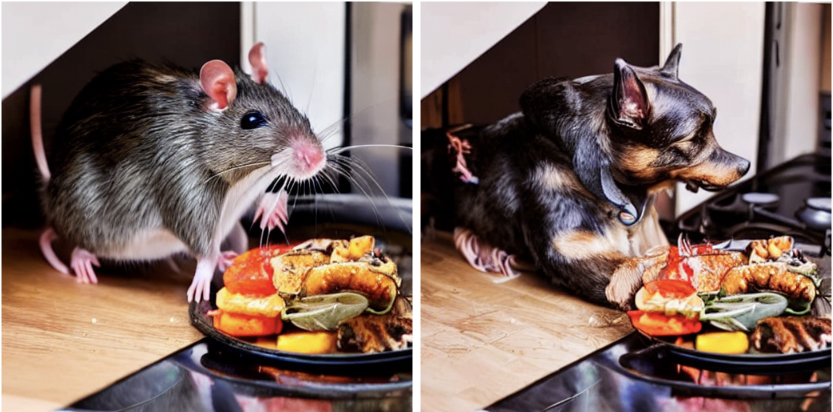 Fig 7: Editing text from “A rat cooking in an apartment” to “A dog cooking in an apartment” with prompt-to-prompt.
We can see in Figure 5 that prompt-to-prompt edits the rat to a dog without changing other features of the photo, as desired. However, we noticed that the result does not give the most natural picture since the dog is looking away and does not look like it is cooking, especially in comparison to the generated image without prompt-to-prompt in Figure 4. This is often the case, and demonstrates one of the limitations with prompt-to-prompt editing, where it may not reach the accuracy of a real picture or a newly generated photo from scratch.
Refinement Editing
In addition to replacement editing, we explored refinement editing, where we change the image by adding an additional word/descriptor to the prompt. We experimented with the prompt “A painting of a rat cooking in an apartment,” and refined it by adding “watercolor” to get “A watercolor painting of a rat cooking in an apartment.” The results are showin Figure 8.
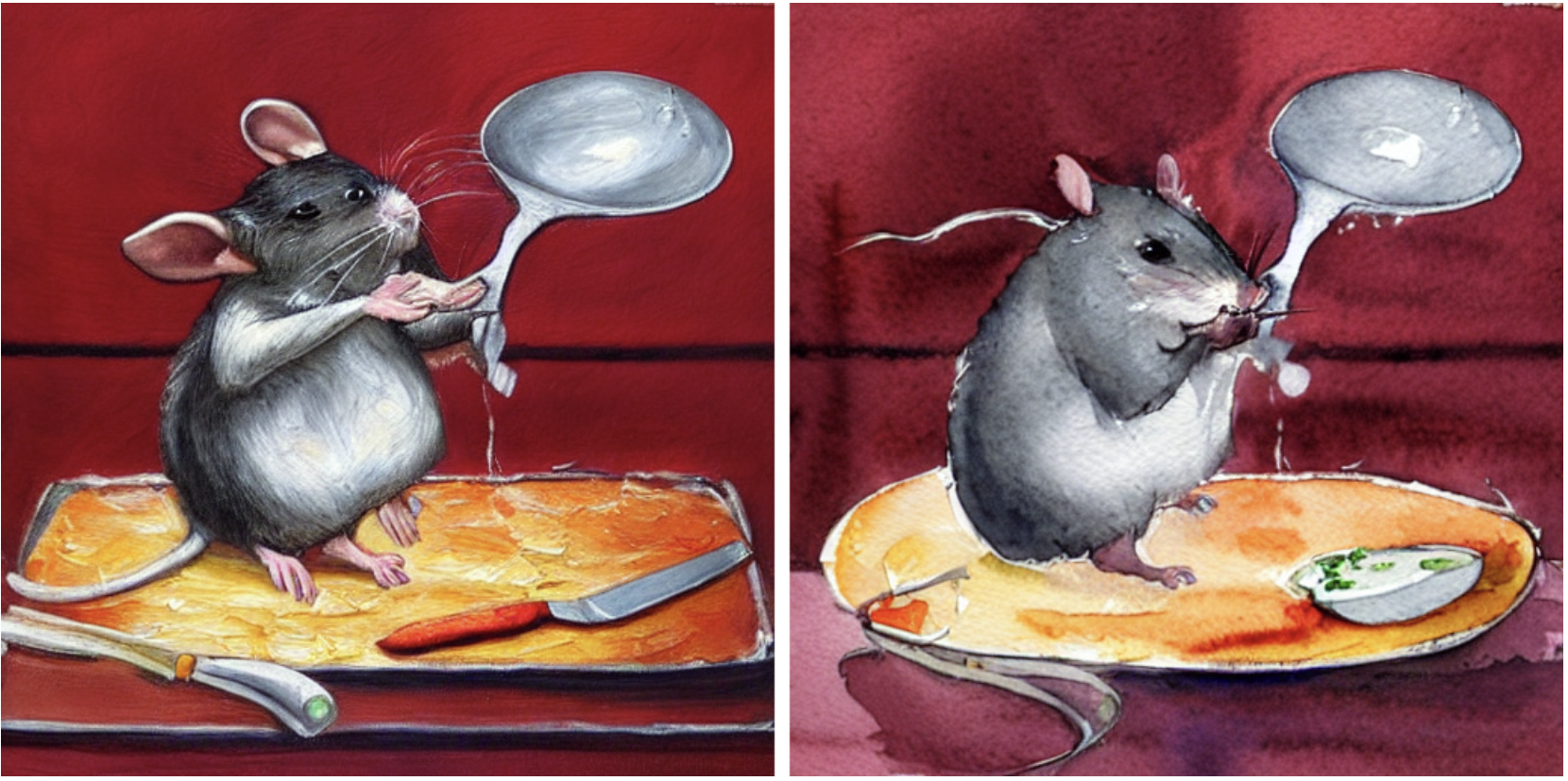 Fig 8: Editing text from “A painting of a rat cooking in an apartment” to “A watercolor painting of a rat cooking in an apartment.”
From the results, we can see that the refinement edit is very well done and fulfills exactly what we requested from the prompt. Refinement editing is quite versatile in adding more detail and changing the overall style of the photo, as seen in this example.
Attention Reweighting
Another aspect of refinement we experimented with was attention reweighting, where we reweight the attention to specific words in order to increase their influence in the output image. We specifically experiment with the prompts “road” and “bumpy road”, and call greater attention to the word “bumpy” to increase its effects on the output image. Figure 9 shows the output without attention reweighting and Figure 10 shows the output with reweighting.
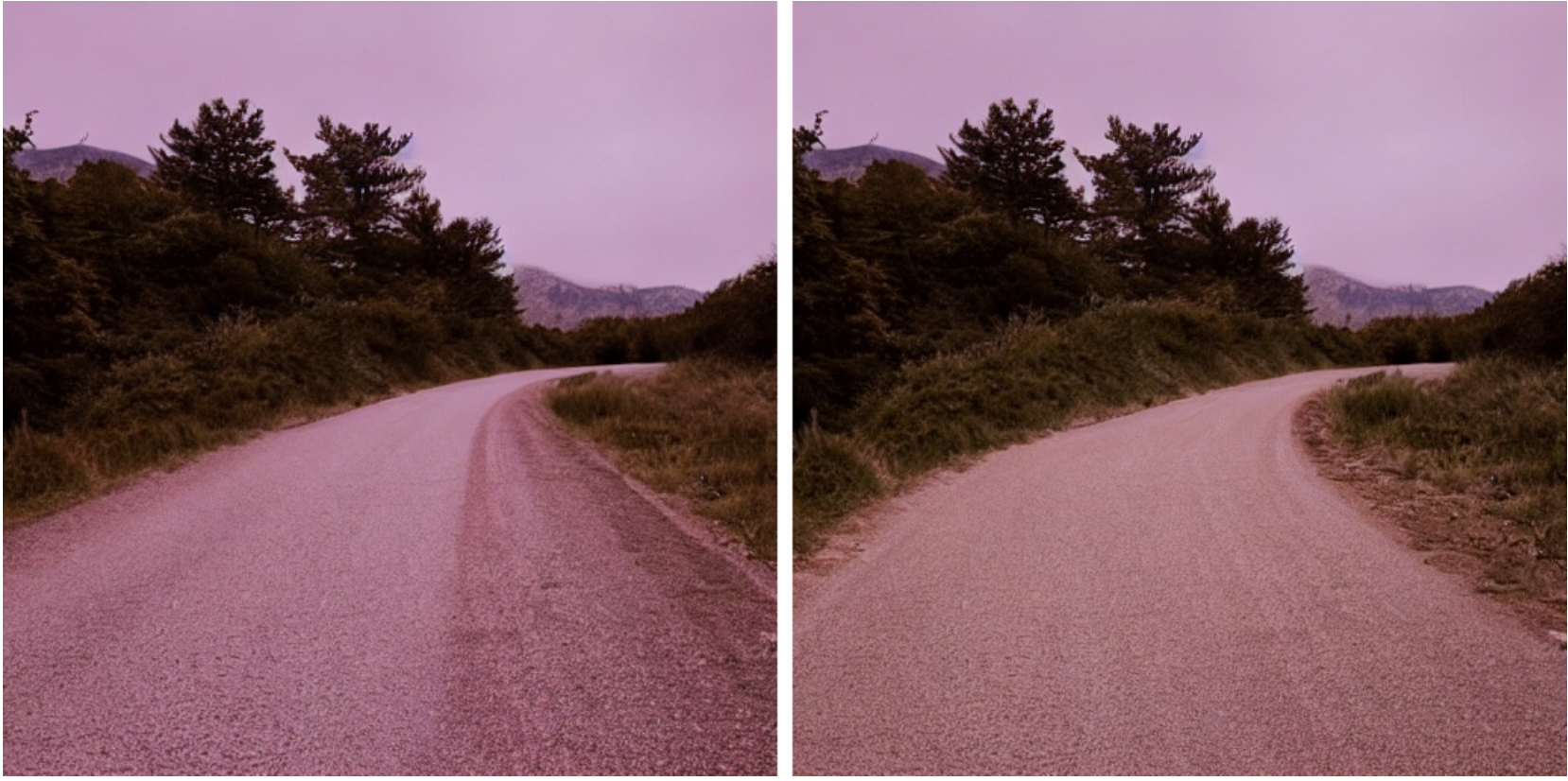 Fig 9: Refinement edit from “road” (left) to “bumpy road” (right) without attention reweighting. The refined image has slightly more bumps, although it is not very noticeable.
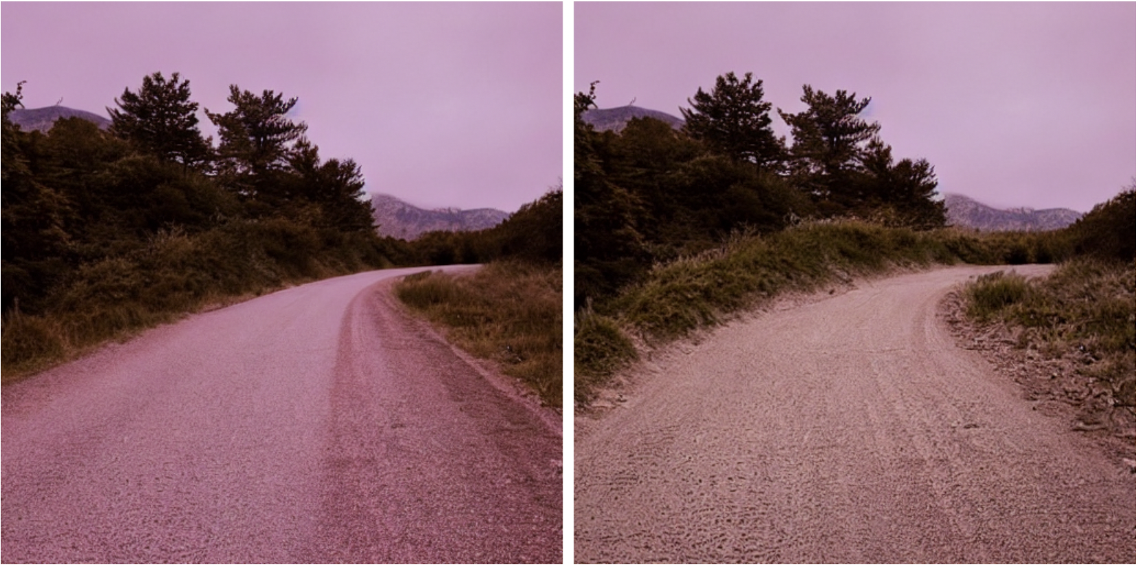 Fig 10: Refinement edit from “road” (left) to “bumpy road” (right) with attention reweighting on “bumpy”. The bumps are much more noticeable in the refined (right) image compared to in Figure 7.
Through this example, we see the power of reweighting attention for a given prompt. Without reweighting, we sometimes get images that do not depict words in the prompt or do not emphasized them as much. By calling attention to specific words through the attention maps mentioned earlier, users have significantly more control over how the image will turn out. However, it is important to note that we must be careful with the amount of attention added when reweighting since if too much weight is added, image details may be uneven and we may lose focus of others features.
Finetuning
Finetuning is the practice of taking a model that has already been trained on a diverse dataset, then training it on a more specific dataset to, in a way, manipulate outputs towards that specific dataset. Here, we explore the finetuning of the Stable Diffusion model on a pokemon dataset, which will make the given text prompts generate pokemon-like images.
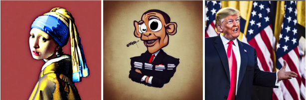 Fig 11: Stable Diffusion outputs for the prompts girl with a pearl earring, cute Obama creature, and Donald Trump before finetuning.
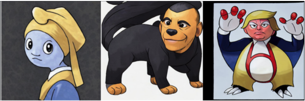 Fig 12: Stable Diffusion outputs for the prompts girl with a pearl earring, cute Obama creature, and Donald Trump after finetuning.
We observe that in Figure 11, without finetuning, the outputs are realistic and what we would expect for the given prompts. They are representative of the dataset with which Stable Diffusion is trained on. With finetuning, however, we see that the generated images are much more pokemon-like for the same exact prompts (Figure 12). The changes are quite drastic, yet remain consistent with the specified prompt, just with a different flavor. This simple sample alone shows the power of finetuning in deep learning.
A consideration when it comes to finetuning is the tradeoff between how closely the generated image follows the given prompt versus the dataset we seek to finetune on. If we train for too short of a time, the generated image will have barely changed from the standard Stable Diffusion output. If we train for too long, the image becomes too much like the dataset and begins to diverge from the prompt.
We can witness this phenomenon for the example prompt “yoda”:
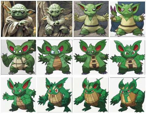 Fig 13: Generated images as the model is finetuned for the prompt “yoda”.
As training continues, the generated image becomes increasingly like the dataset which the model is being finetuned on. However, we observe that the images start to stray from the given prompt. In Figure 13, the final images becomes much like a pokemon, yet we would struggle to identify it as yoda. On the flip side, the first few images are very clearly images of yoda, yet we wouldn’t know it was supposed to be like a pokemon. Finding this balance is a primary concern when it comes to finetuning, hence the importance of logging output images and stopping training when appropriate.
Demo
To set up your environment for finetuning, we recommend cloning the following repository which is a fork of stable diffusion, as it has been setup to be more finetuning friendly.
git clone https://github.com/justinpinkney/stable-diffusion.git
cd stable-diffusion
pip install --upgrade pip
pip install -r requirements.txt
pip install huggingface_hub
You will need to select a dataset containing image and text columns on which to train on. We made use of lambdalabs/pokemon-blip-captions.
from datasets import load_dataset
ds = load_dataset("lambdalabs/pokemon-blip-captions", split="train")
sample = ds[0]
display(sample["image"].resize((256, 256)))
print(sample["text"])
We also need to load the Stable Diffusion model weights from which we want to start finetuning from. We utilize huggingface for this. This is the key element to fine tuning, as we are not training the model from scratch, but from a pretrained state.
from huggingface_hub import login

login()
from huggingface_hub import hf_hub_download
ckpt_path = hf_hub_download(repo_id="CompVis/stable-diffusion-v-1-4-original", filename="sd-v1-4-full-ema.ckpt", use_auth_token=True)
Next, configure the following parameters based on your GPU setup.
BATCH_SIZE = 4
N_GPUS = 2
ACCUMULATE_BATCHES = 1
Finally, we can train the model. You will need to modify the .yaml file to use your own dataset.
!(python main.py \
    -t \
    --base configs/stable-diffusion/pokemon.yaml \
    --gpus "$gpu_list" \
    --scale_lr False \
    --num_nodes 1 \
    --check_val_every_n_epoch 10 \
    --finetune_from "$ckpt_path" \
    data.params.batch_size="$BATCH_SIZE" \
    lightning.trainer.accumulate_grad_batches="$ACCUMULATE_BATCHES" \
    data.params.validation.params.n_gpus="$NUM_GPUS" \
)
Once training is complete, sample the model outputs as so:
!(python scripts/txt2img.py \
    --prompt 'robotic cat with wings' \
    --outdir 'outputs/generated_pokemon' \
    --H 512 --W 512 \
    --n_samples 4 \
    --config 'configs/stable-diffusion/pokemon.yaml' \
    --ckpt 'path/to/your/checkpoint')
Thanks to LambdaLabsML for the example.
Societal Impact
By reducing the cost of training and inference, Stable Diffusion helps democratice the exploration of text-to-image models for all. While there are many positives to this, at the same time, it makes it easy to create and spread malicious data and images. In particular, the deliberate manipulation of images (deepfakes) is a common problem.
Furthermore, as a general text-to-image diffusion model, Stable Diffusion can mirror biases and conceptions that are present in its training data. Such biases can confound assessments of model effectiveness or even be used with bad intent, so data selection must be done with care.
As models like become increasingly powerful, there is a greater need to use them responsibly and carefully. It is incredible to see what Stable Diffusion can already accomplish, and the coming years will no doubt bring even more exciting advancements to this technology.
Conclusion
Our experiments with Prompt-to-Prompt editing and finetuning on Stable Diffusion shows its power and limitations. For Prompt-to-Prompt, although an image generated via Replacement Edit may appear unnatural, the ability to specifically edit and enhance parts of an image via replacement edit and attention reweighting remains a powerful tool. We were impressed by how well the model performed and consider our experiment a success. For finetuning, we were also satisfied with the results. The finetuned model was able to closely abide by the prompt while still giving the appearance of the finetuned dataset (pokemon). Our finetuning experiment demonstrates the further potential of Stable Diffusion, as it can be finetuned on any dataset to generate an image of any theme.
Code
Stable Diffusion Codebase: Github
Prompt-to-Prompt Codebase: Github
Finetuning Experiments: Github
Prompt-to-Prompt Demo: Colab
References
[1] Rombach, Robin, et al. “High-Resolution Image Synthesis with Latent Diffusion Models” Proceedings of the IEEE/CVF Conference on Computer Vision and Pattern Recognition. 2022.
[2] Ho, et al. “Denoising diffusion probabilistic models.” NIPS, 2020.
[3] Hertz, Amir, et al. “Prompt-to-prompt image editing with cross attention control.” arXiv preprint arXiv:2208.01626 (2022).
[4] Esser, Patrick, Robin Rombach, and Björn Ommer. “A note on data biases in generative models.” arXiv preprint arXiv:2012.02516 (2020).