Dataset Analysis for Deepfake Detection Using Mesonet
Abstract
Deepfake detection models and algorithms are the future in preventing malicious attacks against entities that wish to use deepfakes to circumvent modern security measures, sway the opinions of groups of people, or simply to deceive other entities. This analysis of a deepfake detection model can potentially bolster our confidence in future detection models. At the core of the effectiveness of every model is the data used to train and test the model. Good data (generally) creates better models that are more trustworthy to be deployed in real applications. In this study, the MesoNet model is used as the model for training and testing and evaluation. From the three datasets we investigated, the model trained on Dataset 1 (found in Dataset Control) performed the best. We then chose various properties of an image to analyze to compare the three datasets, which include RGB colors, contrast, brightness, and entropy. After comparing the mean and standard deviation across the image properties, we found that the mean values from Dataset 1 are in between the other two datasets and has higher variance in 2 of the 4 image properties observed.
- Abstract
- Spotlight Video
- 1. Introduction & Objective
- 2. About MesoNet and Model Design
- 3. Model Setup and Preparation
- 4. Method: Study Procedure & Algorithm
- 5 Colab Demo & Summary
- References
Spotlight Video
Spotlight Video.
1. Introduction & Objective
1.1 Introduction to Deepfakes and Detection
Deepfakes are videos of a human subject where the person’s facial features are altered or swapped with another person’s face in order to “change” a person’s identity. One common application is videos where a person’s face is exchanged for another such that it seems as though another person is speaking (also known as identity manipulation)[4]. The technology has been developed and improved to the point where deepfaked videos and images may be completely indistinguishable from their real counterparts. They are developed using GANs highly sophisticated minimax methods [3]. This technology is highly deceptive and may pose as a severe security, so researchers are working on deepfake detection: a method to determine whether a given sample is or is not a deepfake. In essence, deep learning has paved the way for deepfakes, but along the same vein, measures need to be created to to ensure that the technology can be limited.
1.2 Objective
In this study, we will be using MesoNet (see next section for more detailed information about the model) to improve deepfake detection holistically. The quality of the data used to both train and test deep learning models is vital to their ability to perform in real world scenarios where deepfake detection is crucial to security and integrity.
One primary objective of this study is to explore existing deepfake datasets and other image datasets based on their effectiveness in use with MesoNet. This is done by training and testing MesoNet on datasets and evaluating its performance using statistics. Model performance will be compared across different datasets.
Another primary objective is to then take the datasets that caused MesoNet to perform well and perform statistical analyses on these datasets to find commonalities or shared characteristics between them. The goal is to uncover whether there are certain traits that may be correlated to better performance with the MesoNet model. Characteristics such as color distribution, contrast, brightness, and entropy are to be used to make these observations. In this way, developers of deepfake detection models in the future may be informed of factors to be watchful of when using datasets to develop their own models.
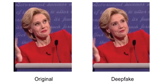
Fig 1. Sample deepfake original (left) and deepfake (right) [1].
2. About MesoNet and Model Design
2.1 How Deepfakes are Created
Deepfakes are generated using auto-encoders, where data is compressed using a shared encoder to reduce computational complexity. To restore the original data, the compressed data is passed through a decoder. In order to create a deepfake, an image is restored according to the decoding of the compressed version of another image [1].
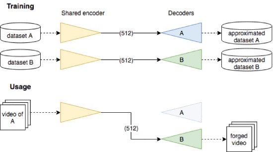
Fig 2. Deepfake Generation Using Encoders and Decoders [1].
2.2 How MesoNet is Designed
The development of MesoNet resulted in two architectures that produced the best classification scores using a low number of parameters. In this study, we will be focusing on Meso-4. Meso-4 is designed with four convolution blocks with one hidden layer. Both ReLU and Batch Normalization are used, and Dropout is used in the fully-connected layers [1].
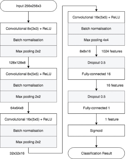
Fig 3. Meso-4 Architecture [1].
For more information, please refer to https://ieeexplore.ieee.org/document/8630761
3. Model Setup and Preparation
3.1 Environment Setup
In order to use MesoNet, the models dependencies need to be taken care of, along with the model’s code. Google Colab will serve this end well with built-in editors and already pre-installed dependencies such as pip. The MesoNet code, authored by Darius Afchar, can be found at the link https://github.com/DariusAf/MesoNet.git.
- Open a new Google Colab project and initialize the runtime.
-
Download the MesoNet code from GitHub and
cdinto the code directory.!git clone https://github.com/DariusAf/MesoNet.git %cd MesoNet -
Load the dependencies of the MesoNet code into Google Colab so that each
.pyfile can recognize other Python files in the same environment (there are dependencies).%load pipeline.py %load classifiers.py !pip3 install face_recognition -
Try running the MesoNet code to make a prediction using the following:
!python example.py
If done correctly and without modifications, the output of this should result in outputting a certain accuracy related to the pre-existing test images in the MesoNet directory. Ignore any errors that are related to videos.
Now your environment is ready to run real data.
3.2 Running the Model on MesoNet’s Data
At this point, we want to be able to check that MesoNet indeed works with test data, which will drive the rest of this study. Sample data can be found at the link https://github.com/MalayAgr/MesoNet-DeepFakeDetection with the Google Drive link as follows: https://drive.google.com/drive/folders/15E6NZr9vhsOfX_nkOtiYkIpWZwtpNi_7.
- Upload the data to Google Drive.
- Access the data.
from google.colab import drive drive.mount('/content/drive') !ls "/content/drive/My Drive/Colab Notebooks/data" - Position the data to be ready for consumption by MesoNet.
# Create new data folder under /content/MesoNet !rm -r test_data !cp -r "/content/drive/My Drive/Colab Notebooks/data/test" "./" !mv "./test" "./test_data" # Rename forged folder to df !mv "./test_data/forged" "./test_data/df" !ls test_data - For the purposes of using this new data, we are going to modify the example Python script to now process the amount of data that is used in this trial dataset.
import numpy as np from classifiers import * from pipeline import * import os, os.path from tensorflow.keras.preprocessing.image import ImageDataGenerator # 1 - Load the model and its pretrained weights classifier = Meso4() classifier.load('weights/Meso4_DF.h5') # 2 - Minimial image generator df_path = './test_data/df' real_path = './test_data/real' df_count = len(os.listdir(df_path)) real_count = len(os.listdir(real_path)) data_count = df_count + real_count print("DATA COUNT:", data_count) dataGenerator = ImageDataGenerator(rescale=1./255) generator = dataGenerator.flow_from_directory( 'test_data', target_size=(256, 256), batch_size=data_count, class_mode='binary', subset='training') # 3 - Predict X, y = generator.next() print('Predicted :', classifier.predict(X), '\nReal class :', y) accuracy = classifier.get_accuracy(X, y) print("Accuracy:", accuracy) # 4 - Prediction for a video dataset # classifier.load('weights/Meso4_F2F.h5') # predictions = compute_accuracy(classifier, 'test_videos') # for video_name in predictions: # print('`{}` video class prediction :'.format(video_name), predictions[video_name][0]) -
Test MesoNet using this new code in order to process the new test images.
!python example.py - The output should look something similar to the following (excluding any progress bars or warnings.
 Predicted : [[0.11766662]
  [0.5160726 ]
  [0.98258865]
  ...
  [0.04207275]
  [0.9486434 ]
  [0.05716746]]
 Real class : [0. 1. 1. ... 0. 1. 0.]
 Accuracy: [0.06616845726966858, 0.9172236323356628]
From here we can see that MesoNet has output predictions between 0 and 1 where 0 means a deepfake image while 1 means a real image. The associated true labels are listed in “Real class” and the Accuracy scores are listed below (note that for index 0, the closer to 0 means the more accurate MesoNet is with classifying deepfakes. Similarly for index 1, the closer to 1 means the more accurate MesoNet is with classifying real images).
At this point, we are ready to run our benchmark study on MesoNet using the model itself.
4. Method: Study Procedure & Algorithm
4.1 Procedure Description
In order to conduct this study, multiple datasets are required to compare the effectiveness of each dataset in training this MesoNet model. Each dataset will be tested as follows.
- Split the dataset into real images and fake sets of images such that binary classification training can proceed.
- Use the
fitfunction of the MesoNet classifier which calls thetrain_on_batchmethod to train MesoNet using the train split of the dataset. - Use a constant control test set in order to check the accuracy of the model upon a test set that the newly trained model has not seen before.
- Repeat this for all the available datasets.
- Discover why certain datasets seem to cause MesoNet to perform better on the test dataset by exploring the features of the training datasets. Use statistical analysis of image properties such as color, lighting, shadows, etc.
4.2 Training and Testing MesoNet
The training data was uploaded to GitHub and can be accessed through the following code.
# TRAIN THE MODEL ON NEW IMAGES
%cd ..
!git clone https://github.com/zachang890/188Data.git
The structure of the data reveals three separate datasets from three different sources that were all used to train MesoNet in separate instances such that MesoNet can be tested fairly across the different datasets. The names of the datasets are Dataset_Control (which contains the first train dataset as well as the test dataset used to evaluate MesoNet), Dataset_2 (which contains the second train dataset), and Dataset_3 (which contains the third train dataset).
Next, we need to write code such that MesoNet can be trained using these datasets. The code used is able to do binary classification training on the Fake and Real data in the function train_Meso4. Training the models using the new datasets (on three separate instances) should take approximately 10-15 minutes per dataset.
Lastly, we need to have code to test MesoNet on some data such that the training datasets can be evaluated for their effectiveness. This is accomplished in the function test_Meso4 where the parameter test_path can always be set to the path that corresponds to the Test directory inside Dataset_Control.
import numpy as np
from classifiers import *
from pipeline import *
import os, os.path
import sys
from tqdm import tqdm
import torch
import tensorflow as tf
from tensorflow.python.client import device_lib
from keras import backend as K

from tensorflow.keras.preprocessing.image import ImageDataGenerator


def train_Meso4(dataset_path_arg, batch_size=64):

  # 1 - Load the model and its pretrained weights
  classifier = Meso4()
  # SETUP TRAIN
  dataset_path_train = os.path.join(dataset_path_arg, 'Train')

  df_count_train = len(os.listdir(os.path.join(dataset_path_train, 'Fake')))
  real_count_train = len(os.listdir(os.path.join(dataset_path_train, 'Real')))
  data_count_train = df_count_train + real_count_train

  # GENERATOR OF TRAIN DATA
  dataGenerator = ImageDataGenerator(rescale=1./255)
  train_generator = dataGenerator.flow_from_directory(
          dataset_path_train,
          target_size=(256, 256),
          batch_size=batch_size,
          class_mode='binary',
          subset='training')

  # TRAIN MODEL USING TRAIN DATA
  epochs = int(data_count_train / batch_size)
  for i in tqdm(range(epochs)):
    train_x, train_y = train_generator.next()
    temp_output = classifier.fit(train_x, train_y)
  return classifier


########################################################

def test_Meso4(classifier, test_path):
  # SETUP TEST
  dataset_path_test = os.path.join(test_path, 'Test')

  df_count_test = len(os.listdir(os.path.join(dataset_path_test, 'Fake')))
  real_count_test = len(os.listdir(os.path.join(dataset_path_test, 'Real')))
  data_count_test = df_count_test + real_count_test
  data_count_test = 100 # Use to avoid over-usage of cpu
  print("DATA COUNT TEST:", data_count_test)

  # GENERATOR OF TEST DATA
  dataGenerator = ImageDataGenerator(rescale=1./255)
  generator = dataGenerator.flow_from_directory(
          dataset_path_test,
          target_size=(256, 256),
          batch_size=data_count_test,
          class_mode='binary',
          subset='training')

  # PREDICT
  X, y = generator.next()
  print('Predicted :', classifier.predict(X), '\nReal class :', y)

  accuracy = classifier.get_accuracy(X, y)
  print("Accuracy:", accuracy)
Below is a sample to run the train and test MesoNet.
# TRAIN
dataset_path_arg = "/content/188Data/Dataset_2"
classifier1 = train_Meso4(dataset_path_arg)

# TEST
test_Meso4(classifier1, "/content/188Data/Dataset_Control")
4.3 Results: Train and Test Results & Interpretation
As mentioned above, MesoNet was trained with a dataset and subsequently tested with a singular test set across three training datasets such that the model can effectively evaluate the datasets. From the training and testing, we achieve the following results.
For Dataset 1 (Found in Dataset Control): [0.161, 0.800] From here, because 0.161 is close to 0.0 (perfect deepfake detection) we can say that the first dataset produced a model that is good at detecting deepfakes. In addition, because 0.800 is close to 1.0 (perfect real image detection) we can say that the dataset produced a model that is good at detecting real images.
For Dataset 2: [0.394, 0.529] From here, because 0.394 is fairly far from 0.0 relative to 0.5 (50/50 chance of deepfake or real), we can say that the second dataset produced a model that is fairly average at detecting deepfakes. In addition, because 0.529 is far from 1.0 and closed to 0.5 we can say that the dataset is not effective at allowing MesoNet to detect real images.
For Dataset 3: [0.377, 0.519] From here, because 0.377 is again fairly far from 0.0 relative to 0.5, we can say that the second dataset produced a model that is fairly average at detecting deepfakes. In addition, because 0.519 is again far from 1.0 and closed to 0.5 we can say that the dataset is not effective at allowing MesoNet to detect real images.
These results are promising for allowing a deeper exploration. One dataset promises more accuracy than the other two which is an open door to investigating why some dataset features may be more effective than others.
4.4 Image Dataset Analysis
Now that we have the accuracy due to each of the datasets, we are now able to perform analysis on each of the datasets to ascertain characteristics that are relevant to comprising a good dataset for MesoNet use. For our analysis, we chose to investigate an image’s average RGB colors, contrast, brightness, and entropy [2].
Definitions
Average RGB colors refers to the color resulting from taking the average color of all pixels in the image. Contrast refers to the difference between the highest and lowest intensity of an image. Brightness refers to the measure of intensity of an image. Entropy refers to the number of bits required to encode image data, which means that images with higher entropy are more detailed.
Implementation Details
We wrote four separate functions to calculate or extract the image properties. The code is shown below. We used libraries like cv2, skimage, PIL, and numpy.
import matplotlib
import cv2
import numpy as np
import skimage.measure
from PIL import Image, ImageStat

def get_rgb(path):
  im_cv = cv2.imread(path) # cv2.imread reads as bgr
  src_img = cv2.cvtColor(im_cv, cv2.COLOR_BGR2RGB)
  average_color_row = np.average(src_img, axis=0)
  average_color = np.average(average_color_row, axis=0)
  return average_color

def get_contrast(path):
  # read image
  img = cv2.imread(path)
  # convert to LAB color space
  lab = cv2.cvtColor(img,cv2.COLOR_BGR2LAB)
  # separate channels
  L,A,B=cv2.split(lab)
  # compute minimum and maximum in 5x5 region using erode and dilate
  kernel = np.ones((5,5),np.uint8)
  min = cv2.erode(L,kernel,iterations = 1)
  max = cv2.dilate(L,kernel,iterations = 1)
  # convert min and max to floats
  min = min.astype(np.float64)
  max = max.astype(np.float64)
  # compute local contrast
  a = max-min
  b = max+min
  # contrast = (max-min)/(max+min)
  contrast = np.divide(a, b, out=np.zeros_like(a), where=b!=0)
  # get average across whole image
  average_contrast = 100*np.mean(contrast)
  return average_contrast

def get_brightness(path):
   im = Image.open(path).convert('L')
   stat = ImageStat.Stat(im)
   return stat.mean[0]

def get_entropy(path):
  im_cv = cv2.imread(path) # cv2.imread reads as bgr
  return skimage.measure.shannon_entropy(im_cv)
Next, we wrote a function to loop through the images in a dataset, size specified by input parameter sample_size, and for each image, extract all 4 properties. Then, we take the average and standard deviation across all of the images.
import os
import numpy as np

# Return averaged image statistics in a dictionary
def get_average_image_stats(dataset_path, sample_size):
  # Initialize
  rgb_arr = []
  contrast_arr = []
  brightness_arr = []
  entropy_arr = []

  # Loop through files in directory
  filenames = os.listdir(dataset_path)
  for i in tqdm(range(sample_size)):
    filename = filenames[i]
    f = os.path.join(dataset_path, filename)
    # Check that it's a file
    if os.path.isfile(f):
      # Get image data
      rgb = get_rgb(f)
      contrast = get_contrast(f)
      brightness = get_brightness(f)
      entropy = get_entropy(f)
      # Append to arrays
      rgb_arr.append(rgb)
      contrast_arr.append(contrast)
      brightness_arr.append(brightness)
      entropy_arr.append(entropy)
  # Convert arrays to numpy
  rgb_arr = np.array(rgb_arr)
  contrast_arr = np.array(contrast_arr)
  brightness_arr = np.array(brightness_arr)
  entropy_arr = np.array(entropy_arr)
  # Average out all stats using numpy
  rgb_arr_mean = np.mean(rgb_arr, axis=0)
  contrast_mean = np.mean(contrast_arr)
  brightness_mean = np.mean(brightness_arr)
  entropy_mean = np.mean(entropy_arr)
  # Standard Deviation
  rgb_arr_std = np.std(rgb_arr, axis=0)
  contrast_std = np.std(contrast_arr)
  brightness_std = np.std(brightness_arr)
  entropy_std = np.std(entropy_arr)
  # Prepare and return result
  result = {}
  result['Average RGB'] = rgb_arr_mean
  result['Average Contrast'] = contrast_mean
  result['Average Brightness'] = brightness_mean
  result['Average Entropy'] = entropy_mean
  result['STD RGB'] = rgb_arr_std
  result['STD Contrast'] = contrast_std
  result['STD Brightness'] = brightness_std
  result['STD Entropy'] = entropy_std
  return result
For our dataset analysis, we set the sample_size to be 1000.
4.5 Results: Dataset Analysis Results & Interpretation
For both Fake and Real images, we compare both the mean and standard deviation of the image properties across all three datasets.
Dataset Fake
Mean
| Dataset | RGB | Contrast | Brightness | Entropy |
|---|---|---|---|---|
| Dataset 1 | [121.207, 97.160, 85.910] | 20.787 | 103.073 | 7.406 |
| Dataset 2 | [92.016, 73.192, 61.838] | 16.079 | 77.517 | 6.856 |
| Dataset 3 | [131.398, 107.393, 95.647] | 24.438 | 113.237 | 7.558 |
Standard Deviation
| Dataset | RGB | Contrast | Brightness | Entropy |
|---|---|---|---|---|
| Dataset 1 | [34.535, 33.427, 34.483] | 8.539 | 32.701 | 0.443 |
| Dataset 2 | [33.378, 27.867, 28.753] | 6.627 | 29.327 | 0.688 |
| Dataset 3 | [29.974, 28.137, 30.072] | 9.295 | 27.850 | 0.287 |
Comparing the means, we see that all the values from Dataset 1 are consisently in between the values from Dataset 2 and Dataset 3. Dataset 2 tends to have consistently lower values while Dataset 3 tends to have consisently higher values across all properties. Comparing the standard deviations, we see that values from Dataset 1 are between values from Dataset 2 and Dataset 3, for contrast and entropy. However, the RGB variance is higher in Dataset 1 than the other 2 datasets so we know that the images in Dataset 1 vary in color more than the images from Dataset 2 and 3. In addition, the standard deviation for brightness in Dataset 1 is higher than both values from Dataset 2 and Dataset 3. Since the standard deviation for brightness is higher, we know that the Fake images in Dataset 1 have higher variance and is more spread out so there are more images with varying brightness and RGB colors than the Fake images in Dataset 2 and Dataset 3.
From our analysis, we can conclude that Dataset 1 has the most variance in RGB colors and brightness in images, Dataset 2 has the most variance in entropy, and Dataset 3 has the most variance in contrast.
Dataset Real
Mean
| Dataset | RGB | Contrast | Brightness | Entropy |
|---|---|---|---|---|
| Dataset 1 | [117.640, 97.900, 88.699] | 20.573 | 102.759 | 7.351 |
| Dataset 2 | [106.991, 88.099, 72.785] | 13.626 | 91.995 | 7.090 |
| Dataset 3 | [134.189, 108.911, 96.894] | 24.040 | 115.105 | 7.587 |
Standard Deviation
| Dataset | RGB | Contrast | Brightness | Entropy |
|---|---|---|---|---|
| Dataset 1 | [36.668, 35.264, 36.689] | 8.527 | 34.685 | 0.471 |
| Dataset 2 | [27.964, 25.828, 22.217] | 5.432 | 25.762 | 0.504 |
| Dataset 3 | [30.312, 28.073, 29.639] | 8.685 | 27.728 | 0.274 |
The observations are similar to the observations made for Fake images. Comparing the means, we see that all values from Dataset 1 are in between the values from Dataset 2 and 3. Dataset 2 tends to have consistently lower values while Dataset 3 has higher values across all properties. Comparing the standard deviations, we see that values from Dataset 1 are between values from Dataset 2 and 3 for contrast and entropy. However, the standard deviation values for RGB and brightness are much higher in Dataset 1 than the other 2 datasets. This means that the Real images in Dataset 1 have higher variance and is more spread out so there are more Real images with different brightness levels and RGB colors than the Real images in Dataset 2 and 3.
Our conclusion is the same for Fake images where we conclude that Dataset 1 has more variance in RGB colors and brightness in Real images, Dataset 2 has the most variance in entropy, and Dataset 3 has the most variance in contrast.
5 Colab Demo & Summary
Here is a link to our Google Colab demo.
In total, these datasets that were used to train MesoNet are an exploratory foray into defining what characteristics of a dataset are most useful to MesoNet to make it an effective deepfake detector. We have found that Dataset 1 which has higher variance in two of the four categories tested where Dataset 2 and 3 have less variance overall. This variety in image composition in Dataset 1 is a possible contributor to its greater detection capabilities, which may be a starting point for future research in this area.
References
[1] D. Afchar, V. Nozick, J. Yamagishi and I. Echizen, “MesoNet: a Compact Facial Video Forgery Detection Network,” 2018 IEEE International Workshop on Information Forensics and Security (WIFS), Hong Kong, China, 2018, pp. 1-7, doi: 10.1109/WIFS.2018.8630761.
[2] Nithyananda C R and Ramachandra A C, “Analysis of Image Properties for Classifying Different Images into Clusters (AIPCDIC),” 2016 International Conference on Wireless Communications, Signal Processing and Networking (WiSPNET), Chennai, India, 2016, pp. 1403-1407, doi: 10.1109/WiSPNET.2016.7566367.
[3] Almars, Abdulqader M. Journal of Computer and Communications, pp. 20–35, Deepfakes Detection Techniques Using Deep Learning: A Survey.
[4] Rossler, Andreas, et al. “Faceforensics++: Learning to detect manipulated facial images.” Proceedings of the IEEE/CVF international conference on computer vision. 2019.