Exploring The Effectiveness Of Classification Models In Autonomous Driving Simulators Through Imitation Learning
In this blog, we explore the effectiveness of supervised learning (classification) models that are trained by imitation learning in autonomous driving simulators.
- Preliminaries
- Research Direction
- Environment Setup
- Environment (Map & Agent) Configuration
- Data collection
- Extracting RGB Image With Ground Truth Actions From Metadrive
- Model design
- Defining Our Own Policy
- Visualization and Evaluation
- Results
- Discussion
- Reference
- Code Repository
Overview Backup link: https://youtu.be/MukdkUluzEc
Preliminaries
Driving simulators provide the fundamental platform for autonomous driving researches. By integrating various deep learning or reinforcement learning pipelines and engines, driving simulators facilitate and standardize model training, validation, testing, and evaluation. The iterations in driving simulators have aimed at a better integration of powerful DL/RL platforms and realistic scene simulations.
MetaDrive is a driving simulation platform designed to facilitate the study of generalizable reinforcement learning algorithms. It supports reinforcement learning tasks such as generalizing to procedural generation scenarios, generalizing to real scenarios, driving under safety constraints, and driving in dense traffic. MetaDrive is able to construct an infinite number of different scenarios for driving. It also provides baselines for these RL tasks.
In this project, we study Metadrive, a lightweight driving simulator supporting compositional map generation and a variety of sensory inputs. We investigate the implementation and configuration of the environment generation, as well as agents’ policies, which defines the way they interact with the environment. By gathering FPV camera image and training customized models, we create new policies using RGB image instead of Lidar data and evaluate the performance of agents in various environments.
As said, MetaDrive uses reinforcement learning models, which learns through trial and error, i.e., it receives feedback from the environment based on its actions, such as reward and penalty. It interacts with the environment until it learns the correct actions.
In this project, we train supervised learning models to learn autonomous driving. These models learn from training data, and are given the correct labels for each of the data points. They aim to predict the correct labels as accurately as possible. By training selected supervised learning models, we aim to explore the potentials of supervised learning and see how they compare with reinforcement learning models.
Research Direction
Our goal in this project is to explore the maximum potential of supervised learning, by training a supervised learning model and comparing how its performance matches a particular reinforcement learning (RL) model. We are applying this approach to the application of driving simulator, when we control a vehicle to drive on a road with different scenarios. Specifically, we want to train a model such that with the RGB image of the vehicle’s front view as its input, it can output the correct steering and acceleration values. Our baseline for comparing our performance is the pretrained RL agent in MetaDrive.
We took the following steps to achieve this goal:
- Obtain RGB images and ground-truth actions from the driving simulation process of MetaDrive using the IDM policy.
- Choose a pretrained DL model and use it to train a supervised learning model using the RGB images as inputs and the ground-truth actions as labels.
- Define a policy which uses the trained model to decide the action based on the observation.
- Evaluate the performance of the policy.
Environment Setup
- Create a new virtual environment for Metadrive
conda create --name Metadrive python=3.8 conda activate Metadrive - Install metadrive as instructed here: Metadrive
- Install relevant packages:
conda install pytorch cudatoolkit=11.3 -c pytorch -c nvidia
conda install -c pytorch torchvision
Environment (Map & Agent) Configuration
The environment configuration is explained in the Metadrive Documentation. For testing and concept validation purposes, we configured a fundamental environment with one-lane on each direction, and no traffic except for the agent. The block generation is also limited to Straight(S) and Circular(C). The size of RGM camera image is set to 128*128.
config = dict(
        use_render=True,
        offscreen_render=True,
        manual_control=True,
        traffic_density=0,
        environment_num=100,
        random_agent_model=False,
        start_seed=random.randint(0, 1000),
        vehicle_config = dict(image_source="rgb_camera",
                              rgb_camera= (128 , 128),
                              stack_size=1),
        block_dist_config=PGBlockDistConfig,
        random_lane_width=True,
        random_lane_num=False,
        map_config={
            BaseMap.GENERATE_TYPE: MapGenerateMethod.BIG_BLOCK_SEQUENCE,
            BaseMap.GENERATE_CONFIG: "SCCCSCCC",  # it can be a file path / block num / block ID sequence
            BaseMap.LANE_WIDTH: 3.5,
            BaseMap.LANE_NUM: 1,
            "exit_length": 50,
    })
The resulting generated evironment is shown below:
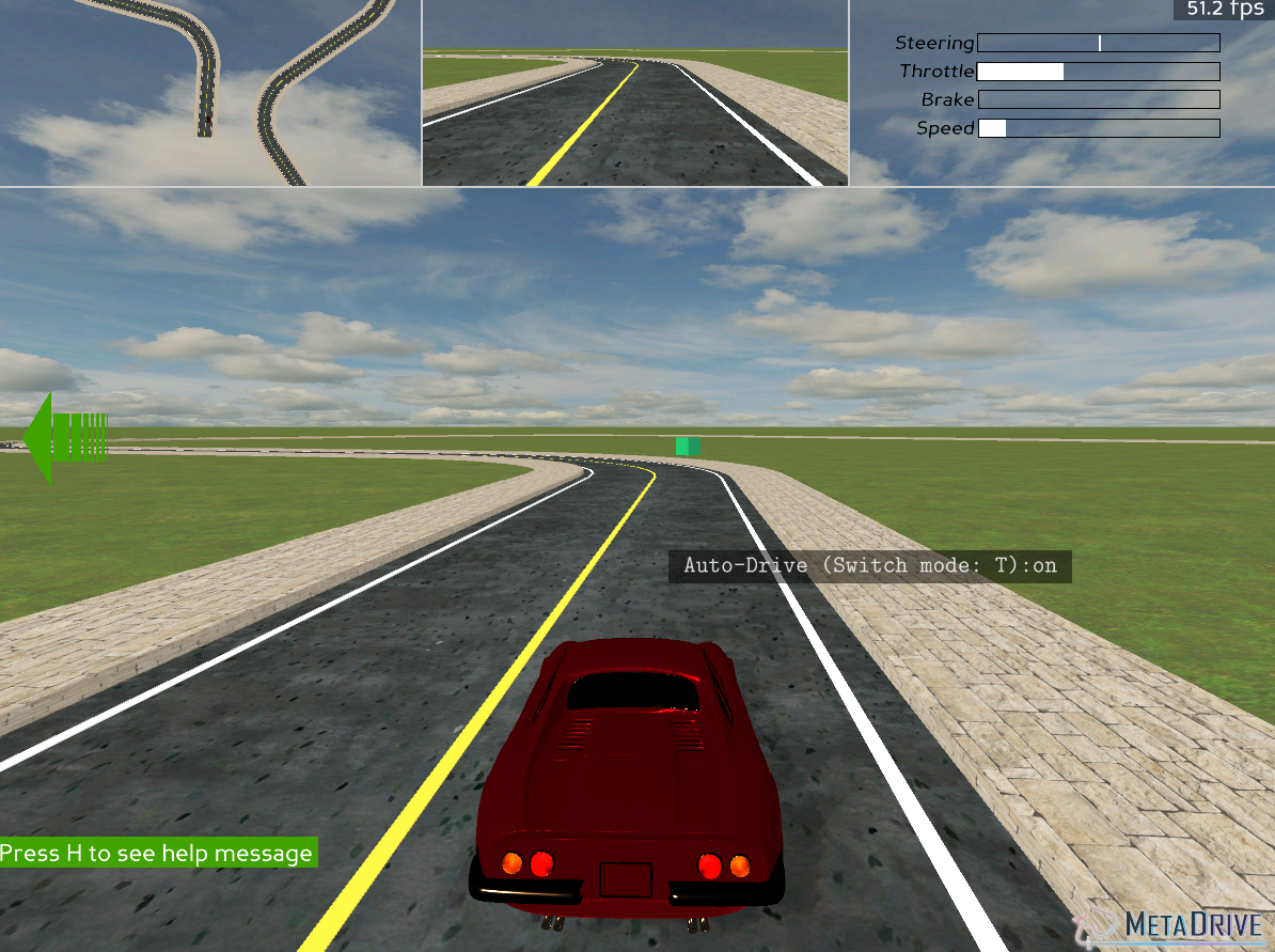 Fig 1. Generated Environment
Data collection
Our training requires a large number of images as training data. To collect this data, we take advantage of the original MetaDrive’s driving policies. During their driving simulation, MetaDrive outputs first-person point of view images. We save these images at an interval of a set number of frames, name these images with the ground-truth actions (i.e., the prediction given by the inherent MetaDrive policy), and use these as the training set. Our data collection process also depends on the tasks we want to train the agent to perform. We next list the scenarios that we targeted.
Single lane, no traffic
The baseline case is the simplest scenario of one traffic lane and no other vehicles on the road. The controlled vehicle only needs to learn to steer when the road ahead curves to the left or to the right.
Single lane, with traffic
The case with one single lane and a certain density of traffic on the road is more complicated. Because the car ahead might be travelling at a lower speed than the controlled vehicle, it must learn to keep a safe distance with the car in the front, which means it has to predict the correct acceleration.
Extracting RGB Image With Ground Truth Actions From Metadrive
In order to train a model that outputs an action space prediction based on the input RGB image, we first need to collect enough images with ground-truth action labeling. To collect these data, we take advantage of the original MetaDrive’s driving policies. During their driving simulation, MetaDrive outputs first-person point of view images. All the data required at this step can be obtained from the obervation and info returned by env.step(). We save these images at an interval of a set number of frames. The action space, as defined in the IDM Policy, consists of two numbers, representing the steering and acceleration respectively. The numbers are used to directly name the image file, which is placed in validation set or training set as configured.
o, r, d, info = env.step([0, 0])
action_space = (info['steering'], info['acceleration'])
if PRINT_IMG and i%SAMPLING_INTERVAL == 0:
    img = np.squeeze(o['image'][:,:,:,0]*255).astype(np.uint8)
    img = img[...,::-1].copy()
    img = Image.fromarray(img)
    root_dir = os.path.join(os.getcwd(), 'dataset', 'val')
    img_path = os.path.join(root_dir, str(action_space) + ".png")
    img.save(str(img_path))
The image obtained, as shown below, contains all the information about the lane that the agent vehicle requires to make a good prediction.
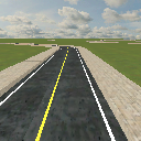 RGB Image Example
Model design
| Method | Model | Traffic | Speed Info | Data Augmentation | Training Data Manipulation | Need manually defined max speed |
|---|---|---|---|---|---|---|
| RN | ResNet | × | × | × | × | ✓ |
| VT | ViT | × | × | × | × | ✓ |
| VT-TT (3 tokens) | ViT | × | × | ✓ | × | ✓ (reduced complexity) |
| VT-SA | ViT | × | ✓ | ✓ | × | × |
| VT-STA | ViT | ✓ | ✓ | ✓ | × | × |
| VT-STM | ViT | ✓ | ✓ | ✓ | ✓ | × |
| SF-A | SlowFast | × | N/A | ✓ | × | × |
| SF-TA | SlowFast | ✓ | N/A | ✓ | × | × |
| SF-TM | SlowFast | ✓ | N/A | ✓ | ✓ | × |
We created several designs for our supervised learning model. For each design, we take a pretrained model (except ViTs), train it using the images we generated, and save the checkpoint model. The table above summarizes the properties of each model we used. We next introduce each of the models we used in detail.
In order to better distinguish and list the models with different designs and training dataset, we name the models using the following conventions:
- VT: base model is ViT; RN: base model is ResNet18; SF: base model is SlowFast
- TT: three tokens (will be explained below)
- S: has speed token input
- T: training data collected in with-traffic environment
- A: data augmentation (grayscale)
- M: training data manipulation
Baseline Resnet And ViT
We used pretrained ResNet18, with no modifications to the input structure. We replaced the final linear layer to ouput a 2-element vector, representing the action space. For ViT, we used the architecture in the assignment. The extra class token is used to predict the final action space, and similarly we replaced the linear layer in the final MLP head to achieve so. However, it’s worth noticing that we have to manually set the acceleration to 0 when the vehicle’s speed exceeds a certain maximum speed, otherwise the ego vehicle simply keeps accelerating.
ViT Three Tokens (VT-TT)
Instead of using one extra token (the class token) for action space prediction, we used three tokens, corresponding to acceleration, steering, and speed respectively. We hoped the three tokens can have attention on each other, and learn to control the speed. Similar to the previous approaches, we still manually imposed the maximum speed limit, but now the max speed came from model predictions.
Slow Fast (SF)
It is rather difficult to capture speed info using image classification models. Slow Fast was thus proposed as an alternative approach as it outputs a classification result based on video, or consecutive frames, as the input. Thus, the input itself can incoporate speed information. Since the input is of a completely different format, we had to recollect all the training data. For each run using the expert policy, we collected every other frame, and we collected 4 runs in total. As a result, we ended up with a training set consisting of ~300 videos.
Data augmentation (-A)
We applied grayscale trasnformation to the images as data augmentation.
Speed Token For ViT (-S)
Although ViT with three tokens can be used to predict the desired speed of the vehicle in every time stamp, it was still not a “fully autonomous” model as we had to manually define a policy, setting the acceleration to zero if the ego vehicle’s speed exceeds the predicted speed. We discovered a caveat of the previous approaches: speed should be a given variable or an input to the model, instead of an output. Thus, we proposed VT-S.
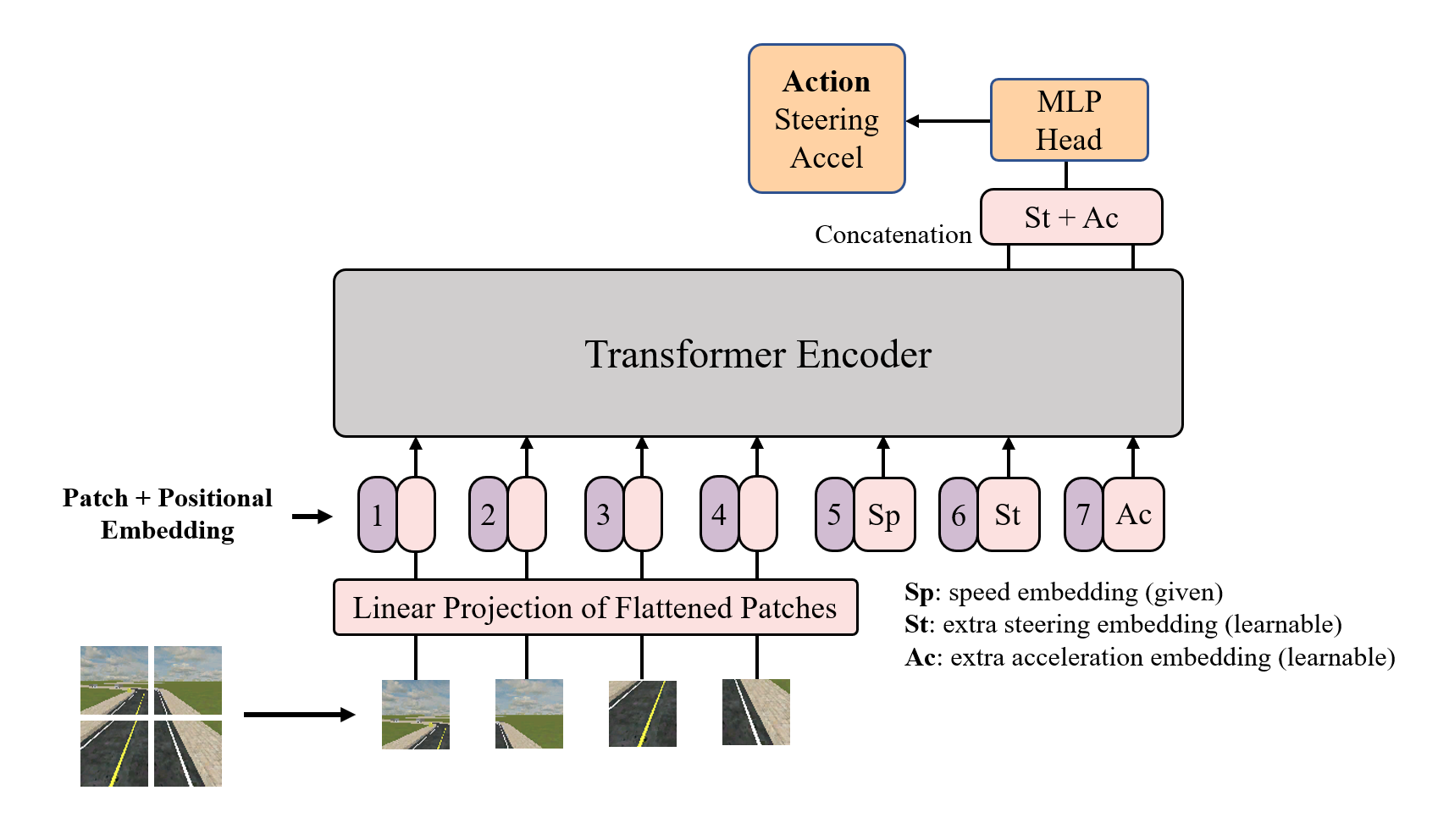 VT-S Diagram
VT-S has three extra tokens. The first one represents the current speed of the ego vehicle. The second and the third token, after the encoder layers, are concatenated and passed into an MLP head to output the final action space, acceleration and steering, prediction. We hope by this design, we can encode the speed information into the model learning & prediction process, and make the model able to establish attention mechanisms between acceleration, steering, and the given speed.
With Traffic (-T)
In addition to the 2K images dataset without traffic, we further added 1.5K images with traffic and trained the best-performing model in no-traffic environment on the new dataset. We hope by this we can extend the usability of the classification model in autonomous driving.
Training Data Manipulation (-M)
Instead of having a training dataset consisting of both no-traffic and with-traffic sitautions, we redesigned the entire dataset to consist only of with-traffic situation. We collected 1K images using fixed-interval sampling, and collected an additional 1K images when the vehicle was braking due to another vehicle in front. By changing the ditribution and adding bias to the dataset, we hoped the model could learn to brake and follow a front vehicle easier.
Training Setup
We defined a dataloader to handle the dataset we collected, which simply reads in the image file and processes its filename to store as the label. Some code implemented are omitted for readability.
class Metadrive(Dataset):
    def __init__(self, root_dir, split, transform=None):
        for path in os.listdir(os.path.join(root_dir, 'dataset', split)):
          if os.path.isfile(os.path.join(root_dir, 'dataset', split, path)):
            self.filenames.append(path)

    def __getitem__(self, idx):
        image_path = os.path.join(self.root_dir, 'dataset', self.split, self.filenames[idx])
        image = Image.open(image_path)
        label = self.filenames[idx][1:-5]
        label = label.split(', ')
        steering = (float(label[0])-steering_mean)/steering_std
        acceleration = (float(label[1])-accel_mean)/accel_std
        return image, torch.Tensor([steering, acceleration])
In order to validate that our implementation for the data loader is correct, we used a pretrained ResNet18 from PyTorch and added a fully connected linear layer at the end, transforming the 512-dim tensor to the 2-dim tensor, which represents the action space we intend to obtain from the model prediction. We set different learning rates for different layers, and we used MSE loss as the criterion since we are dealing with a continuous value prediction model.
optimizer = torch.optim.SGD(model.resnet.fc.parameters(), lr=0.01, momentum=0.9)
for name, param in model.named_parameters():
    if param.requires_grad and 'fc' not in name:
        optimizer.add_param_group({'params': param, 'lr':0.005})

criterion = nn.MSELoss()
Epoch 1/10: 100%|██████████| 15/15 [00:01<00:00, 10.91it/s, loss=5.09e+3]
Validation set: Average loss = 12432554169393362758105300992.0000
Epoch 2/10: 100%|██████████| 15/15 [00:01<00:00, 11.38it/s, loss=1.8e+3]
Validation set: Average loss = 5299107328.0000
Epoch 3/10: 100%|██████████| 15/15 [00:01<00:00, 10.88it/s, loss=11]
Validation set: Average loss = 206780.1484
Epoch 4/10: 100%|██████████| 15/15 [00:01<00:00, 10.42it/s, loss=1.43]
Validation set: Average loss = 6.6199
Epoch 5/10: 100%|██████████| 15/15 [00:02<00:00,  6.32it/s, loss=0.873]
Validation set: Average loss = 1.2147
Epoch 6/10: 100%|██████████| 15/15 [00:02<00:00,  7.08it/s, loss=1.16]
Validation set: Average loss = 1.0740
......
Epoch 10/10: 100%|██████████| 15/15 [00:01<00:00, 10.67it/s, loss=0.769]
Validation set: Average loss = 0.9185
It is worth noticing that before training, we standardize the values of steering angle and acceleration (code shown below). As shown from the above output, the loss decreased noticeably, but the best loss we could obtain stayed at around 0.9 without further improving. The analysis of this result and possible improvements to be done in the future will be discussed in later sections.
def get_mean_std(root_dir):
    steering = []
    accel = []

    for path in os.listdir(os.path.join(root_dir, 'dataset', 'train')):
        if os.path.isfile(os.path.join(root_dir, 'dataset', 'train', path)):
            label = path[1:-5]
            label = label.split(', ')
            steering.append(float(label[0]))
            accel.append(float(label[1]))

    steering = np.array(steering)
    accel = np.array(accel)

    return np.mean(steering), np.std(steering), np.mean(accel), np.std(accel)
Defining Our Own Policy
We defined a policy class named RGBPolicy which inherits from BasePolicy in MetaDrive. Upon initialization, we set self.model to be the trained supervised learning model which we load from a previouly saved checkpoint. We overrode the act() function, so that it obtains an RGB image from the controlled object, converts the image to tensor, and calls the self.model on the tensor to obtain an action (including steering and acceleration). The code is as follows:
class RGBPolicy(BasePolicy):
    PATH = "model.pt"

    def __init__(self, control_object, random_seed):
        super(RGBPolicy, self).__init__(control_object=control_object, random_seed=random_seed)
        self.model = Resnet()
        self.model.load_state_dict(torch.load(RGBPolicy.PATH, map_location=torch.device('cpu')))
        self.model.eval()

    def act(self, *args, **kwargs):
        # get a PNMImage
        img = self.control_object.image_sensors["rgb_camera"].get_image(self.control_object)

        # PNMImage to tensor
        img = self.__convert_img_to_tensor(img)

        data_transform = transforms.Compose([
            transforms.Normalize((0.485, 0.456, 0.406), (0.229, 0.224, 0.225))])
        img = data_transform(img)

        action = self.model(img)[0].detach().numpy()
        return action

    def __convert_img_to_tensor(self, img):
        img = np.frombuffer(myTextureObject.getRamImageAs("RGBA").getData(), dtype=np.uint8)
        img = img.reshape((myTextureObject.getYSize(), myTextureObject.getXSize(), 4))
        img = img[::-1]
        img = img[...,:-1] - np.zeros_like((128,128,3))
        img = torch.from_numpy(img)
        img = img/255
        img = img.permute(2, 0, 1)
        img = torch.unsqueeze(img, 0)
        return img
It is worth noticing that in the above code, we have to unnormalize the values of steering angle and acceleration returned by the model. And we applied a scaling factor to the steering, which is a value determined by emperical trials.
Visualization and Evaluation
Our evaluation involves three steps. Firstly, we train each model we choose and store the checkpoint into a local file. We feed the images we collected from the data collection stage into the model and make it learn the correct labels such as speed, steering and acceleration. Secondly, we define a policy based on the trained model, which loads the checkpoint from the saved file and runs inference with that model to decide which action to take at each step. In other words, the policy is a mapping from the vehicle’s front-view image to its actions. The final step in the evaluation process is to run the driving simulation and observe its performance. The time taken and the cost (an evaluation metric defined by the MetaDrive RL model) are recorded to assess the effectiveness of the model.
Results
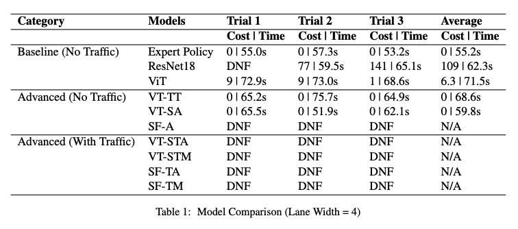 Result for Lane Width = 4
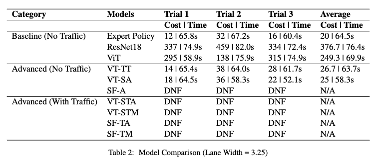 Result for Lane Width = 3.25
Baseline Resnet And ViT
ResNet18 demonstrates the ability of a simple classification model to correctly steer the ego vehicle. However, the high costs and the occasional DNFs show that there is still great potential of classification models.
The basic version of ViT was trained using the same dataset as ResNet. The model immediately showed an improvement from ResNet, demonstrating the effectiveness of the attention mechanism. It achieved an average cost of 6.3 on a lane of width 4, in comparison, ResNet had a cost of 109 (not considering one DNF).
However, a downside of both models is that they failed to properly maintain the speed. The acceleration prediction was always greater than 0. We had to manually impose a maximum speed and set acceleration to 0 accordingly. This was against our purpose of developing a fully autonomous vehicle using classification models.
ViT Three Tokens
Similar to the previous approaches, we still manually imposed the maximum speed limit, but now the max speed came from model predictions. This model was first trained on the baseline 1K images, and achieved a significant improvement with respect to ResNet and baseline ViT. The average cost on width-4 lane was 0, and 120 on width-3.25 lane. We thus further trained the model with the expanded 2K images dataset. The model, again, achieved 0 cost on the wider lane, and a lower 73.3 average cost on the narrow lane.
Data augmentation
After identifying the issue that the model was paying too much attention to the while line on the right of the lane, thus continously crossing the central yellow line, we applied grayscale trasnformation to the images as data augmentation. ViT with three tokens’ performance was further improved. Average cost on the 3.25-width lane decreased to 24.
ViT With Speed Token And Data Augmentation
VT-SA’s performance was promising. Not only it achieved similar low costs as the previous best model, it greatly reduced the time to reach the destination. The average cost on 4-width lane was 0, and the average time was 59.8s. In comparison, ViT with three tokens’ time was 68.5s. VT-SA’s time on 3.25-width lane also decreased from 63.6s to 58.3s.
In addition to the reduced time and cost, VT-SA needed no manually defined policis. It was able to learn to brake when the speed was too fast and when entering a turn. VT-SA model fully demonstrated its capability of manuvering the ego vehicle in an ideal no traffic situation.
ViT With Speed Token In Traffic
In addition to the previous 2K images dataset without traffic, we further added 1.5K images with traffic and trained VT-STA on the new dataset. However, the model became more likely to output noisy acceleration values, such as braking when not necessary. Most importantly, the model was not able to properly brake when a vehicle was in front of the ego vehicle. While the expert policy was able to achieve 0 crash, ours VT-STA constantly crashes.
Training Data Manipulation
As against to our original hope, the result after training data manipulation was that the model could not even properly accelerate the ego vehicle when there was nothing in front. The ego vehicle didn’t even start to move forward, showing that such a dataset manipulation approach completely failed its purpose.
Discussion
Limitation of Classification Model
Autonomous vehicles rely heavily on computer vision models to recognize and interpret the environment around them. Image classification models are commonly used in these systems to identify and classify objects in the scene. However, when it comes to predicting continuous action space values, such as steering angle or speed, these models have limitations. Image classification models are designed to categorize images into a set of predefined classes based on their visual features. These models work by learning the patterns and features in the input images and then using this information to make predictions about the class labels of new images. However, these models have limitations when it comes to predicting continuous action space values. This is because continuous action spaces involve predicting a value that lies on a continuous scale according to a large variety of possible input data. That is to say, action space prediction should be the last component of autonous driving’s pipeline, while classification models are seemingly more suiable for the prior tasks.
Effectiveness of Data Augmentation
Comparing ViT and VT-TT, we can see that for both lane width = 3.25 and lane width = 4 cases, data augmentation helps reduce the cost during evaluation. By converting the images to grayscale, certain details that may be present in the original images, such as color gradients or textures, are removed. This can allow the model to focus more on the overall layout and composition of the image, which may be more important for driving simulation tasks.
Effectiveness of Different Model Designs
Among the models we chose, i.e., ResNet, ViT and SlowFast, ViT proves to be the best-performing model. With the added features such as data augmentation and speed information, its evaluation cost is close to that of the baseline RL expert. ViT greatly improves the performance over the previously-chosen ResNet model. To our disappointment, however, SlowFast is not able to further improve the performance of the driving simulator.
Limitation of SlowFast
As mentioned earlier, the SlowFast model requires learning from sequences of images, or videos, in order to capture the temporal information. During our training, we used 300 videos as the input data. While this is a relatively large dataset, it may not be sufficient for the SlowFast model to learn the correct speed information. This is because the SlowFast model requires a significant amount of data samples to effectively learn the temporal information and capture the relationship between motion and appearance.
Dfficulty of Training Data Collection
As explained in the data collection section, this process can be rather time consuming depending on the coputation power. Additionally, the sampling process of the images inevitablly adds bias to the training data set, as the ground-truth action space at every time frame can be drstaically different. However, collecting every time frame as well leads to overfitting issue. Balancing between the two extremes can be a difficult process, and the data collected eventually determines the performance of the model.
Difficulty of Evaluation
Evaluating the model performances in MetaDrive was a relatively difficult process. While fixing the block sequence or disabling randomness can seemingly establish a fair comparison between models, those approaches may as well introduce bias in situations where a certain model can perform exceptionally well in a apsecific map. Thus, we had to manually test the performance by running the same model in randomly generated maps of the same block sequence several times (three trials per lane width). Due to the computation power limitation, each trial takes a rather long time. Spending too much evaluating the models’ performances has impeded us from extending the project to more realistic environments such as multi-lane maps.
Future Improvements
There are several implementation ideas that we thought of but did not fulfill within the time constraints. For example, we can use model ensembles to aggregate the predictions of different models and improve the performance.
Reference
[1] Q. Li, Z. Peng, L. Feng, Q. Zhang, Z. Xue, and B. Zhou, “MetaDrive: Composing Diverse Driving Scenarios for Generalizable Reinforcement Learning,” arXiv, 2021. doi: 10.48550/ARXIV.2109.12674.
—