Object Detection Algorithms

This project explores different R-CNN based deep learning algorithms used for object detection. We analyze the performance 5 different R-CNN based models for transfer learning on a new dataset, using OpenMMLab’s MMDetection toolbox to finetune these 5 models, pretrained on COCO and using the Aerial Maritime target dataset.

• Introduction
  • What is object detection?
  • Applications of Object Detection
  • Major Milestones in History of Object Detection
• Basic Definitions
  • Convolutional Neural Networks
  • Performance Metrics
  • Transfer Learning
• Model Introduction
  • R-CNN: Regions with Convolutional Neural Networks
  • Fast R-CNN
  • Faster R-CNN
  • YOLO - You Only Look Once
  • Cascade R-CNN
  • Dynamic R-CNN
  • Libra R-CNN
  • Grid R-CNN
  • Model Results on COCO Dataset
  • Models Run on UCLA Photos
• Method
  • Datasets
  • Evaluation Metric
  • Using MMDetection for Transfer Learning
  • Model Training
  • Links to Our Code
• Results and Discussion
  • Training accuracy
  • Training time
  • Inference Time
  • Model weights size comparison
  • Test accuracy results
  • Sample predictions on images
  • Adversarial attacks
• Conclusion
• Video Presentation
• Reference

Introduction

Object detection is an invaluable computer vision task that involves identifying and localizing objects within an image. This project explores different R-CNN based deep learning algorithms used for object detection based on transfer learning performance on a new dataset. We compare 5 R-CNN models (Faster R-CNN, Cascade R-CNN, Dynamic R-CNN, Grid R-CNN, and Libra R-CNN) using OpenMMLab’s MMDetection toolbox. The models are pretrained on the Microsoft COCO dataset and the target dataset consists of aerial maritime images containing objects of 5 classes: car, lift, jet ski, dock, and boat. Cascade, Dynamic, Grid, and Libra R-CNN are variants on Faster R-CNN that all perform better on the COCO dataset. In our project, we aimed to explore how these models perform when finetuned for transfer learning on a new dataset. We hypothesized that Cascade, Dynamic, Grid, and Libra would all perform better than Faster R-CNN on the new dataset because of their enhancements in training. Additionally, we are using pretrained weights for most layers, and only changing the number of classes in the final prediction head. Most results were consistent with our expectations-Cascade, Libra, and Dynamic R-CNN all performed better than Faster R-CNN. However, it was surprising that Grid R-CNN performed worse than Faster R-CNN on our new dataset. We discuss some hypotheses for why this may have occurred. Before analyzing the overall mAP performance on the Aerial Maritime test dataset, we discuss the class-wise performance, training curve, training time, and model size of each model. We visualize a few sample test outputs of each of the models to qualitatively compare the results. Finally, to test the robustness of the different models, we also explore the effects of adversarial attacks.

What is object detection?

Object detection is a computer vision task that requires locating objects in a digital photograph and classifying or identifying them. Given an image as input, the object detection model should output a set of annotations. Each annotation contains the bounding box, represented by a point, width, and height, the class label of the object in this bounding box, and a confidence score indicating the certainty with which the model has classified this object [1]. Figure 1 below shows a sample output of an object detection model. Before the task of object detection, computer vision researchers focused on image classification, that is, classifying an image in one or more categories. Object detection can be considered a more advanced extension of image classification, in which we label specific portions of the image, instead of the entire image. This project explains some major deep learning algorithms used for object detection and reproduces their results using OpenMMLab’s MMDetection toolbox.

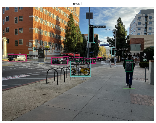
Figure 1: An example output of an object detection algorithm called Grid R-CNN [1].

Applications of Object Detection

Object detection has many applications. Self-driving cars use object detection to detect locations of other cars, pedestrians, traffic signals, and other critical objects on the road. More generally, robots use object detection to view and interact with the world around them. Another use of object detection is to caption images and videos based on the objects in them. This is needed for increasing web accessibility. Facial detection is also a subset of object detection focused on detecting where faces are located in an image. Facial detection is used in cameras, photography, and for marketing. Video surveillance makes use of object detection for security purposes. These are just some of the numerous applications of object detection.

Major Milestones in History of Object Detection

Over the past 25 years, object detection has grown greatly as a field of computer vision research [2]. Figure 2 below shows the number of publications in object detection over time.

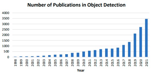
Figure 2. Increase in Number of Object Detection Publications From 1998 to 2001 [2].

The history of object detection can be divided into two eras: pre and post deep learning. Before 2014, object detection was done using traditional methods, including handcrafted, low-level features, and shallow machine learning architectures. After 2014, deep learning became the focus of object detection algorithms research. Here is a list of important object detection milestones, describing how approaches changed over time:

• 2001: Viola Jones Detectors detect human faces in an image by sliding windows of all possible sizes over all locations of the image, and checking whether these windows contained a face, using a machine learning classifier. The researchers incorporated new techniques to speed up performance. Viola and Jones used Haar-like features, commonly used for object detection at the time. Haar-like features are adjacent rectangles that are white and black, or of drastically different intensities, that are used to identify common patterns in images. For example, they are used to detect edges and certain regions of the face like the eyes and nose, that have contrasting dark and light areas. [2] [3]
• 2004: Scale Invariant Feature Transform SIFT is a method to extract features from an image that are invariant to scale and rotation of the image. Using SIFT features, variations in illumination, perspective, and noise does not greatly affect the accuracy of image matching. [4]
• 2005: Histogram of Oriented Gradients (HOG) feature extraction method is proposed, which outperforms other methods including SIFT. [5]
• 2008: Deformable Part-based Model (DPM) was the quintessential traditional object detection model. DPM used a divide-and-conquer approach, called the star-model. It would detect different parts of the object in order to detect the object as a whole. [2]
• 2012: ImageNet classification with deep convolutional neural networks. A deep convolutional neural network is able to learn high-level features automatically. [6]
• 2014: Regions with CNN Features (R-CNN). 2014 saw the start of the Deep Learning Era of Object Detection. Inspired by the use of deep convolutional neural nets for image classification, researchers tried using CNNs for object detection. R-CNN proposed a successful architecture that saw many future improved versions over the next several years. R-CNN is discussed in detail later in this article. [7]
• 2015: Fast R-CNN [8]
• 2015: Faster R-CNN [9]
• 2015: You Only Look Once (YOLO) [10]
• 2015: Single Shot MultiBox Detector [11]
• 2017: Feature Pyramid Networks (FPN) [12]
• 2020: Object Detection with Transformers [13] We will discuss some of the major models, from the deep learning era of object detection, in detail in the Model Introduction section.

Basic Definitions

Convolutional Neural Networks

Before exploring models in depth, we must provide a background to the building blocks and terminology. Convolutional neural networks (CNN) are a class of artificial neural networks that are most commonly applied to analyze visual images. They are specifically designed to process pixel data and the connectivity pattern between neurons is loosely inspired by biological processes resembling the organization of the animal visual cortex. They apply convolution filters, also known as kernels, to an image to produce feature maps. A mathematical operation called a convolution is used in place of general matrix multiplication to generate the layers. The network learns to optimize these filters through automated learning.

A CNN consists of multiple layer elements: an input layer corresponding to the image dataset, convolutional layers where the image becomes abstracted to a feature map, pooling layers to reduce dimensions by combining small clusters, and fully connected layers, which connect every neuron in one layer to every neuron in another layer, and ensure the output is of the desired dimension. In the convolutional layers, each output neuron is based on input from a restricted area of the previous layer called the receptive field.

Figure 3 below shows an example of the convolution operation, applying a 2x2 filter to a 3x3 input. We take the dot product of each 2x2 window of the input with the 2x2 filter to get the 4 elements of the output matrix.

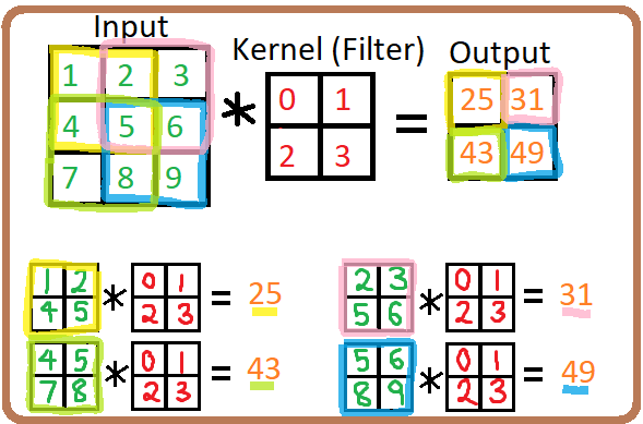
Figure 3. An example of the convolution operation, applying a 2x2 filter to a 3x3 input.

Performance Metrics

Before discussing different object detection algorithms, it is important to discuss the metrics used for evaluating their performance. The standard metric used in object detection research is mean Average Precision (mAP). The terms below help explain how we determine whether a prediction is correct or incorrect, and the mAP metric for model performance.

Precision

Precision is a value representing the percentage of correctly identified objects out of all objects the model identifies. A model with high precision is desirable.

Recall

Recall measures the ability of the model to detect all ground truths, in other words, all objects in the images. A model with high recall is desirable.

Intersection over Union (IoU)

IoU evaluates the degree of overlap between the ground truth and prediction and ranges from 0 to 1, with 0 meaning no overlap and 1 indicating perfect overlap. The IoU of the prediction bounding box, P, and the ground truth bounding box, G, is defined as the area of intersection of P and G areas, divided by the area of union of the P and G areas. Figure 4 below shows a visualization of computing IoU.

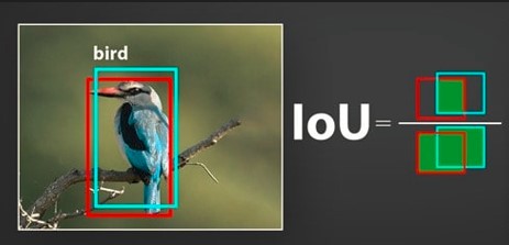
Figure 4. Visualization of Intersection over Union (IoU) Computation [14].

For a given class label, for example bird, if the prediction bounding box and the ground truth bounding have an IoU of greater than 0.5, the prediction is considered correct. Different IoU thresholds (denoted by \(\alpha\)), like 0.75 can be chosen if we want to increase the requirement of overlap for a prediction to be deemed correct. If multiple predictions are made for the same object, the first one is counted as a correct prediction, while the rest are considered incorrect, because it is the job of the algorithm to filter out duplicate predictions of the same object. If the model labels the same bird using 10 different boxes, varying only in location and size, only 1 prediction will be counted as a correct prediction, while the other 9 will be counted as incorrect predictions.

Precision Recall Curve

Precision recall curve is a plot of precision and recall at varying confidence thresholds. Each confidence threshold (not to be confused with IoU threshold \(\alpha\)) is used to determine whether a prediction should be trusted or not. The model outputs a confidence score with each prediction, indicating how confident the model is about this prediction. For a given confidence threshold, we can calculate the precision and recall scores, with only predictions above the threshold considered as positive predictions. If the threshold were 0.70, then a prediction with 0.60 confidence would not be considered as a positive prediction. Each threshold creates a point on the precision recall plot, with many of these points forming the curve.

ROC Curve

A Receiver Operating Characteristic (ROC) curve is a graph showing the performance of a model at all classification thresholds. It plots the two parameters: true positive rate (equivalent to Recall) and false positive rate.

Average Precision (AP)

Average Precision is the area under the precision recall curve. We calculate AP for each class in the dataset. \(AP@\alpha\) denotes an AP that is calculated using an IoU threshold of \(\alpha\).

Mean Average Precision (mAP)

The mean Average Precision is the AP averaged over all classes in the dataset (e.g. classes = [bird, cat, dog, person, car, …]).

To calculate the average precision for the class, bird, in our dataset, we first sort the predictions by their confidence levels. For each confidence level, we calculate the precision and recall scores of all predictions above that confidence level. We plot (recall, precision) points to form a precision-recall curve. The area under the curve gives the Average Precision for the bird class. Then, we find this precision for each class in the dataset, and the mean of all the AP values gives the mean Average Precision, or mAP, of predictions.

Transfer Learning

Transfer learning is the technique of using a pre-trained machine learning model, created for a certain task (called a base task or source task), for a new task (called a target task). The model’s learned weights on the original task are used as a starting point for learning the new task, by using the pretrained weights for weight initialization. Then, training is done specifically configured for the new task to finetune the model, meaning make it perform better on the new task.

Model Introduction

R-CNN: Regions with Convolutional Neural Networks

Motivation

From 2010 to 2012, object detection performance was generally stagnant, with little improvements made by ensemble models [7]. The best models up to this point were made using SIFT and HOG, low-level, engineered features. The R-CNN object detection algorithm resulted in a mAP of 53.3% on the PASCAL VOC 2012 dataset, which was a 30% improvement compared to the previous best performance [7]. In 2012, Krizhevsky et al. [6] showed that using CNNs for image classification resulted in a significant performance improvement. Therefore, researchers explored using CNNs for the task of object detection.

Main Ideas

One main problem to solve in object detection is localization, the task of locating objects in the image. This can be done by treating localization as a regression problem or using a sliding-window approach, both of which have certain issues with performance for deep neural networks. R-CNN uses region proposals, which are bounding boxes of areas of interest in the image, that are suspected to contain an object to be labeled. Given an input image, it generates about 2000 category-independent region proposals, of various sizes, and uses a CNN to create a fixed-length feature vector for each region proposal. Then, each region proposal is classified using class-specific linear SVMs. The combination of CNNs and region proposals explains the model’s name, R-CNN. Figure 5 below illustrates this process at a high level.

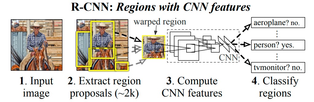
Figure 5. R-CNN steps at a high level [7].

Another major problem to solve is the insufficient amount of labeled data for training a large CNN. One solution to this problem is to do unsupervised pre-training, and then supervised fine-tuning. The R-CNN paper proposes using supervised pre-training on a large auxiliary dataset, and then domain-specific fine-tuning on a small dataset, as a successful method of training deep CNNs when lacking adequate training data.

R-CNN consists of 3 parts:

1. Generate Category-Independent Region Proposals. R-CNN is compatible with many different region proposal methods, but uses selective search for this paper. Selective search combines aspects of exhaustive search and segmentation to create a stronger region proposal algorithm. It uses a bottom-up approach, finding many small, separate areas of the image, then combining them in a hierarchical manner to find the final region proposals. While this is not a deep learning algorithm, it is still important for region proposals in object detection.

2. Use CNN to Extract a Fixed-Length Feature Vector From Each Region Proposal. A CNN is used to create a 4096-dimensional feature vector from each region proposal. A mean-subtracted 227x227 RGB image is forward propagated through 5 convolutional layers and 2 fully connected layers. To convert the region proposal, an arbitrary sized image, to a 227x227 image, warping is used to resize the image. To do testing, the test image goes through selective search to produce about 2000 region proposals, which are then fed through the CNN to produce feature vectors.

3. Class-Specific Linear SVMs Used for Classification of Region Proposals. Finally, each feature vector is scored by each class-specific SVM, indicating the likelihood of the region proposal being in the SVM’s class. For each class, duplicates are removed by rejecting boxes that overlap largely with a higher scored box.

Efficiency of R-CNN

Because the only class-specific step is step 3, the method outlined by R-CNN is very efficient. The CNN model parameters are shared across classes, and the CNN creates a relatively small feature vector (4K dim). The computation of region proposals and feature vectors is only done once, shared by all classes. The feature matrix is 2000x4096, with 2000 region proposals each encoded as a 4096 feature vector. The SVM weight matrix is 4096xN, since there is a separate SVM for each of N classes.

Training the R-CNN using Innovative Approach

Pre-training of the CNN was done using the auxiliary dataset, containing only image-level labels, not bounding box information. Then, the CNN model parameters are used as initializations for the domain-specific CNN training. To fit the CNN to our object detection task, as opposed to image classification, the CNN’s classification layer is modified to be for N+1 classes, where N is the number of object classes and +1 is for the background class, instead of the unrelated class size of the image classification dataset. We use the warped region proposals to complete the training of the CNN. For the Stochastic Gradient Descent, each mini-batch during training contains 32 positive warped region proposals and 96 background ones, in order to favor the positive windows, which are the minority group. This supervised pre-training on a large auxiliary dataset and then domain-specific fine-tuning on a small dataset was an innovative approach that tackled the issue of a lack of training data.

Summary

Overall, R-CNNs were a major breakthrough in improving object detection model performance by introducing a method of applying CNNs to region proposals, and a method of training with limited object detection data by using auxiliary image classification data.

Fast R-CNN

Fast R-CNN trains and predicts faster and with higher accuracy than R-CNN. In R-CNN, the generated region proposals are too general, therefore, after the SVMs do classification, a bounding-box regression stage is used to make the bounding boxes more precise [8]. Training the SVMs and bounding-box regressor is expensive in both compute time and space in memory because of the large feature vectors representing the region proposals.

Fast R-CNN aims to simultaneously learn to classify region proposals and refine the object localizations in its fully connected layers. Fast R-CNN training can be done in a single-stage and updates all the network layers, uses a multi-task loss, and requires no disk storage for feature caching.

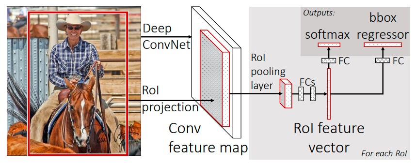
Figure 6. Fast R-CNN Architecture [8].

The main difference in Fast R-CNN is that the entire image is passed through the CNN to get a feature map representing the entire image. This is very different from R-CNN, where each region proposal is passed through the CNN to get features for the region proposals. This difference means that Fast R-CNN requires less passes through the CNN, feeding-forward once per image, instead of 2000 times per image, assuming there are 2000 region proposals for an image. For a given image, for each object proposal, a fixed-length feature vector is extracted from the feature map of the image. This is done by a Region of Interest (RoI) pooling layer.

These feature vectors are then passed through some fully connected layers, and split to result in two outputs. One split goes through softmax to give the vector probabilities of the region proposal being in each of the classes and the additional background class. The other outputs the bounding boxes for each class, using per-category bounding-box regressors. Figure 6 above shows the Fast R-CNN architecture.

Faster R-CNN

Faster R-CNN further improves the train and prediction time of the object detection model by introducing Region Proposal Network (RPN) instead of pre existing region proposal algorithms such as Selective Search and EdgeBoxes [9]. These pre-existing methods were found to be bottlenecks, accounting for at least half of the inference time in state-of-the-art object detection models. Figure 7 shows the architecture of Faster R-CNN.

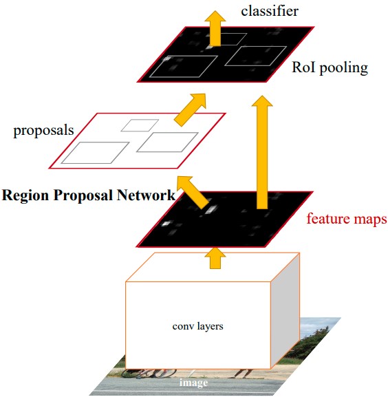
Figure 7. Faster R-CNN Architecture [9].

Two main contributions of Faster R-CNN are:

1. Region Proposal Network (RPN) The RPN is a deep convolutional neural network to compute the region proposals for a given image. It shares its layers with the CNN used in R-CNN and Fast R-CNN to compute the features. This sharing means that the RPN does not add significant time to the total inference time, because it uses the computation that already needed to be done to get the convolutional feature map. The RPN takes an image as input, and outputs a set of region proposals, each with an objectness score representing how likely the region is to contain any object, as opposed to it being in the background class.

2. Anchor Boxes Faster R-CNN introduces anchor boxes to generate rectangular region proposals of different shapes and sizes. Using a fixed-size sliding window over the convolutional feature map, each window is passed through classifier and bounding-box regressor. At each sliding window location, multiple region proposals are predicted, with various scales and aspect ratios. We call these anchor boxes, because they are boxes centered at the sliding window’s center, called the anchor. Figure 8 below shows the RPN and visualizes the anchor boxes given the current sliding window position.

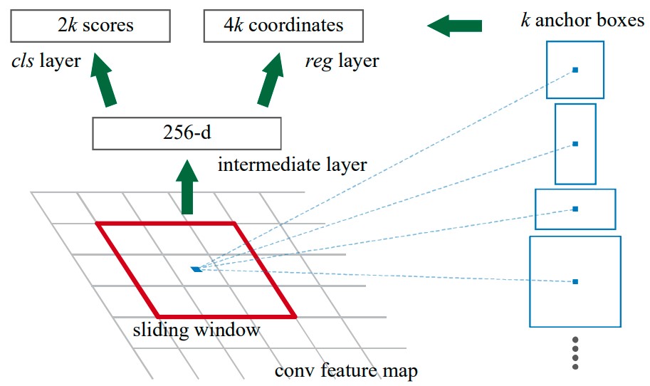
Figure 8. Faster R-CNN’s Region Proposal Network with Anchor Boxes [9].

YOLO - You Only Look Once

R-CNN and its improved versions are two-stage object detection algorithms. There exists popular single-stage algorithms such as YOLO and Single Shot MultiBox Detector. We did not explore these models in this project as we wanted to compare only variants of R-CNN, but found it important to understand the model. The YOLO (You Only Look Once) algorithm is a real-time object detection framework first introduced in 2015. It identifies spatially separating labeled bounding boxes which correspond to rectangular shapes around the objects. It has gone through multiple improvements through the years with YOLOv7 (released in 2022) making significant improvements in the field. The latest version, YOLOv8, was released in January 2023.

The YOLO algorithm divides the input image into a grid of cells and predicts the bounding boxes and class probabilities for each cell [15]. Each bounding box contains a predicted object location and its corresponding class probability. The YOLO framework has 3 main components. The backbone extracts essential features and feeds them to the head through the neck and is composed of convolutional layers. The neck collects feature maps and creates feature pyramids. The head consists of output layers that have final detections.

YOLOv2 introduced the use of anchor boxes which are predefined shapes of different aspect ratios and scales that are used to predict the bounding boxes of objects within an image. Feature pyramid networks (FPN) were introduced in YOLOv3. Each new version of YOLO introduced the use of larger backbone networks, and improvements in accuracy through different techniques such as different ways to better generate anchor boxes. A key improvement in YOLOv7 is the use of a new loss function called “focal loss” as opposed to a standard cross-entropy loss function used in previous versions [16]. YOLOv7 made a major change in the architecture and used the trainable ‘bag-of-freebies’ model, allowing the model to improve the accuracy without increasing the training cost. YOLOv7 has a high resolution, and its main advantage is its fast inference speed along with a high average precision.

Cascade R-CNN

Cascade R-CNN is a variant of Faster R-CNN, introduced in 2018 by Microsoft Research Asia. It aims to solve the problem of degrading performance as IoU thresholds increase [17]. This problem stems from overfitting during training and inference-time mismatch between the IoUs for which the detector is optimal and those of the input hypotheses. The model uses a multi-stage object detection architecture: a sequence of detectors trained with increasing IoU thresholds, sequentially trained with the output of each detector as training data for the following detector. This is designed so that the last detector has the highest recall, lowest false positive rate of the sequence. The resampling of progressively improved hypotheses guarantees that all detectors have a positive set of examples of equivalent size, reducing the overfitting problem. The same cascade procedure is applied at inference. This model performs particularly well on datasets with high levels of occlusion and clutter. Figure 9 shows the difference in architecture between Faster R-CNN and Cascade R-CNN ((a), (d) respectively in Figure 9).

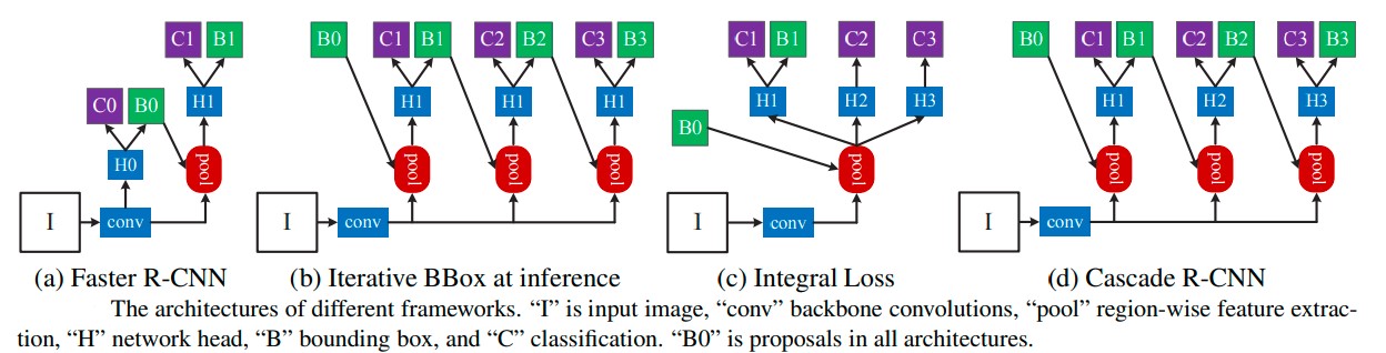
Figure 9. Architecture of different frameworks: (a) Faster R-CNN (b) Cascade R-CNN [17].

Dynamic R-CNN

Dynamic R-CNN is a variant of R-CNN, introduced in 2019 by Facebook AI Research. It aims to improve performance by dynamically adapting the network architecture to the input image [18]. In the training process, a fixed label assignment strategy and regression loss function can’t fit distribution change of proposals which can be harmful to training high quality detectors. Dynamic introduces dynamically adjusted IoU Threshold for label assignment and by dynamically adjusting shape of regression loss function (dynamic SmoothL1 Loss). Both dynamic settings are based on the distribution of proposals during training. Dynamic SmoothL1 Loss involves computing dynamic weights for each object proposal based on its size and aspect ratio, then computing the loss by taking the difference between target and predicted values and multiplying by the dynamic weights. Figure 10 illustrates the dynamic label assignment process. Dynamic R-CNN is good for datasets with high levels of variation in object size, aspect ratio, and lighting conditions.

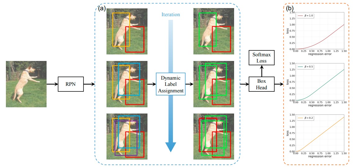
Figure 10. Dynamic R-CNN, dynamic label assignment and loss [18].

Libra R-CNN

Libra R-CNN is a variant of Faster R-CNN, introduced in 2019 by Facebook AI Research. It aims to address the problem of class imbalance in the training process by introducing balance at the sample level, feature level, and objective level [19]. There are 3 novel components: IoU-balanced sampling, balanced feature pyramid, and balanced L1 loss, respectively for reducing the imbalance at sample, feature, and objective level. The IoU-balanced sampling approach ensures the model sees an equal number of positive and negative examples for each class. The model dynamically adjusts sampling probabilities for each class based on their current training performance, with underrepresented classes being given a higher weight. In traditional models, features extracted from the image are often misaligned with ground truth bounding boxes leading to localization errors. The Libra model aligns extracted features with ground truth bounding boxes by first estimating offsets between features and bounding boxes, then warping features to align using bilinear interpolation. This makes the model good for detecting small objects. The Libra model also uses a balanced L1 loss which promotes gradients accurate samples to rebalance the involved tasks and samples. This improves the model robustness to small variations in object position and scale, leading to improved localization accuracy. Figure 11 shows a high-level overview of the architecture.

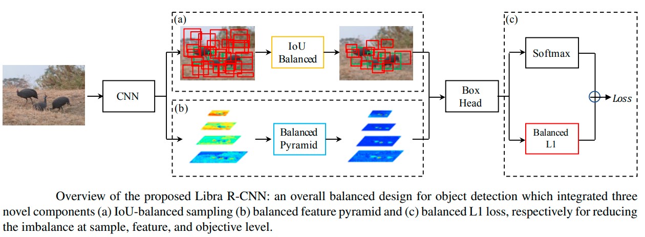
Figure 11. Libra R-CNN architecture [19].

Grid R-CNN

Grid R-CNN is a variant of Faster R-CNN, introduced in 2019 by the Facebook AI Research team. It uses a grid guided approach to find the bounding boxes, instead of using a regression approach to better model the spatial relationships between different parts of an image [20]. It uses a fully convolutional neural network to do localization, instead of the traditional sequence of fully connected layers. The core idea of this model is to divide the input image into a grid of smaller regions, then process each of these regions independently using a modified version of Faster R-CNN. Other innovations were also implemented to improve performance: a new feature fusion technique that combines features from different levels of a convolution neural network and multi-task learning. In Faster R-CNN, the features from the backbone network are typically pooled to a fixed size and then passed through a region proposal network (RPN) and a detection head. However, this pooling operation discards a lot of spatial information and can result in a loss of localization accuracy. Grid R-CNN, features from different levels of the backbone network are combined to generate a set of multi-scale feature maps. Features are combined from different levels in a way that preserves spatial information. It is then used to generate region proposals. In Faster R-CNN, the RPN and detection head are trained independently which may negatively impact performance as the two tasks are related and can benefit from shared knowledge. In Grid R-CNN, the RPN and detection head are trained jointly using a single loss function, allowing for information sharing. This model is particularly helpful when objects are densely packed together or partially occluded. Figure 12 shows an overview of the pipeline of Grid R-CNN.

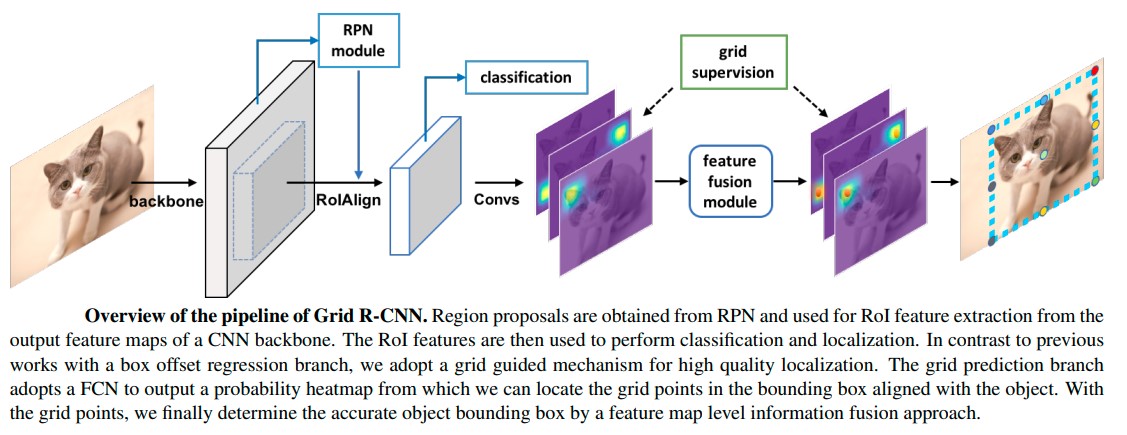
Figure 12. Grid R-CNN Pipeline [20].

Model Results on COCO Dataset

In our project, we are analyzing the following 5 R-CNN based models: Faster R-CNN, Cascade R-CNN, Dynamic R-CNN, Grid R-CNN, and Libra R-CNN. First, let us examine the results of these 5 models on the COCO 2017 dataset, which was used to pretrain them. It is important to understand this first, in order to later compare these results to the results after transfer learning on the Aerial Maritime dataset (the new/target dataset). We used the following config and model files to load the pretrained models’ settings and weights. We will discuss these selected models in more detail in the Methods section.

rcnn_links = {
    "faster": {"model": "https://download.openmmlab.com/mmdetection/v2.0/faster_rcnn/faster_rcnn_r50_fpn_1x_coco/faster_rcnn_r50_fpn_1x_coco_20200130-047c8118.pth", 
               "config": "./configs/faster_rcnn/faster_rcnn_r50_fpn_1x_coco.py"},
    "cascade": {"model": "https://download.openmmlab.com/mmdetection/v2.0/cascade_rcnn/cascade_rcnn_r50_fpn_1x_coco/cascade_rcnn_r50_fpn_1x_coco_20200316-3dc56deb.pth",
                "config": "./configs/cascade_rcnn/cascade_rcnn_r50_fpn_1x_coco.py"},
    "dynamic": {"model": "https://download.openmmlab.com/mmdetection/v2.0/dynamic_rcnn/dynamic_rcnn_r50_fpn_1x/dynamic_rcnn_r50_fpn_1x-62a3f276.pth",
                "config": "./configs/dynamic_rcnn/dynamic_rcnn_r50_fpn_1x_coco.py"},
    "grid": {"model": "https://download.openmmlab.com/mmdetection/v2.0/grid_rcnn/grid_rcnn_r50_fpn_gn-head_2x_coco/grid_rcnn_r50_fpn_gn-head_2x_coco_20200130-6cca8223.pth",
                "config": "./configs/grid_rcnn/grid_rcnn_r50_fpn_gn-head_2x_coco.py"},
    "libra": {"model": "https://download.openmmlab.com/mmdetection/v2.0/libra_rcnn/libra_faster_rcnn_r50_fpn_1x_coco/libra_faster_rcnn_r50_fpn_1x_coco_20200130-3afee3a9.pth",
                "config": "./configs/libra_rcnn/libra_faster_rcnn_r50_fpn_1x_coco.py"},
}

Figure 13 below shows the mAP of each of the 5 models on the COCO dataset. As expected, Libra, Dynamic, Cascade, and Grid R-CNN perform better than Faster R-CNN because each added various improvements to Faster R-CNN, as explained earlier. Grid R-CNN performs the best with an mAP of 0.404, Libra R-CNN performs second worst with mAP of 0.383, and Faster R-CNN performs worst with mAP of 0.374. Cascade and Dynamic R-CNN perform second and third best, with mAPs of 0.403 and 0.389 respectively.

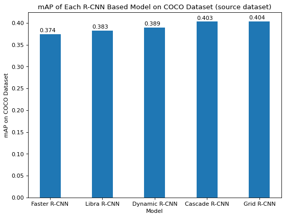
Figure 13. mAP of Each R-CNN based Model on COCO.

Models Run on UCLA Photos

We ran these 5 models on images from UCLA and the surrounding area. The figures below show results on different images. The objects detected are only objects part of COCO’s 80 classes, including person, traffic light, car, backpack, and truck. We will discuss each image’s results in detail now.

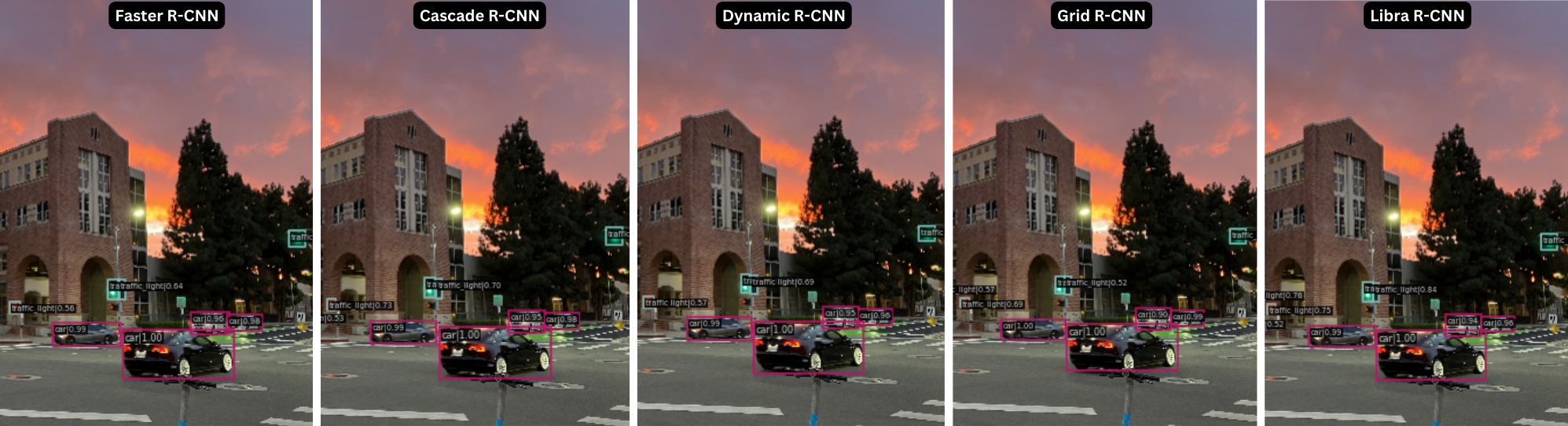
Figure 14

In Figure 14, all of the R-CNN models correctly detect the 4 cars in the image. They also correctly detect 2 traffic lights in the center of the image, and 1 at the right edge of the image. However, the models all incorrectly detect a traffic light on the left edge of the image, which is actually a pedestrian crossing LED showing a red/orange hand. It makes sense that this looks like a traffic light because from a distance, it looks like a red circle, not a hand.

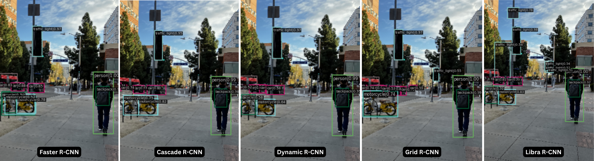
Figure 15

From Figure 15 above, the most notable result was that it is difficult for the models to detect a bike in a bike rack due to occlusion. There is just 1 motorcycle in the bike rack, but it is detected as two objects by all models except Grid R-CNN. This is consistent with the result from Figure 13 that Grid R-CNN performs best out of the 5 pretrained models we selected to use.

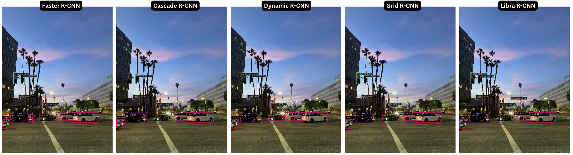
Figure 16

All the models perform fairly similarly in Figure 16. For instance, they all detect the cars quite well, except they all misclassify the black car near the left side of the image as a truck, with moderate confidence. There are some differences, nevertheless. Cascade R-CNN fails to detect a traffic light that is behind the Left Turn Only/No U-Turn sign, but all other models do correctly detect this, showing their robustness to occlusion. Libra R-CNN is the only model to incorrectly detect a palm tree in the background as a traffic light.

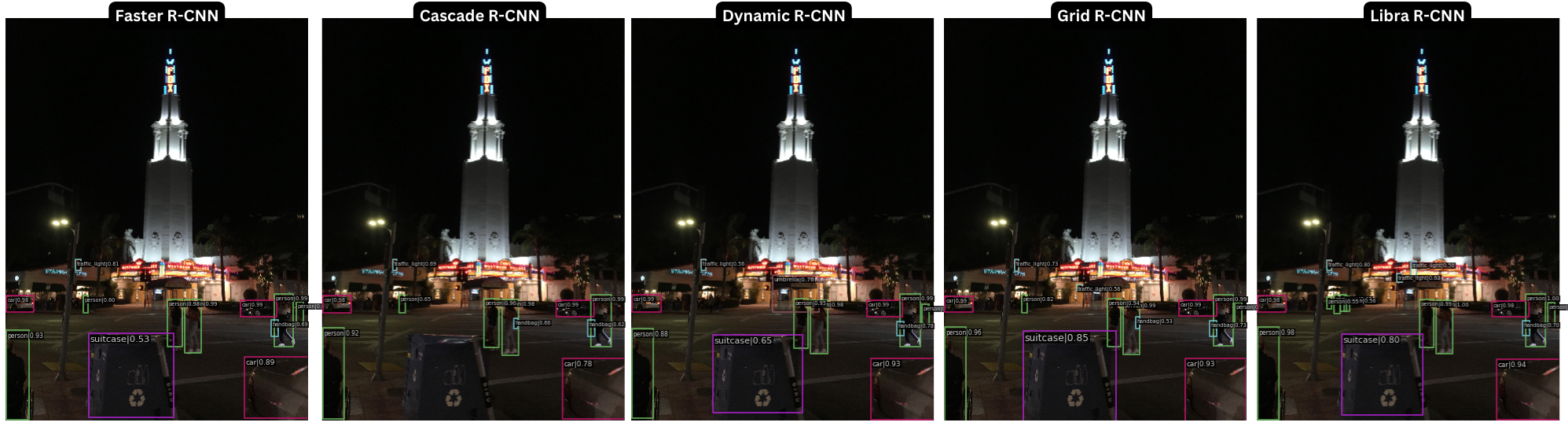
Figure 17

Figure 17 was particularly interesting because it was taken at night. We were interested to see if the models would be able to detect the people in the dark, thinking it may be challenging for the models. However, the models performed very well. They all detected the people and cars in the scene, and even detected the car in the bottom right corner of the image, based on just the tiny portion of the car that was showing in the image. Another observation is that Cascade R-CNN was the only model that did not detect the recycling bin as a suitcase. All the other models detected the recycling bin as a suitcase, though it does not have a handle like a suitcase would, and is not perfectly rectangular like a suitcase. Looking at the class wise APs of the models, I see that the suitcase has an AP of 0.35 to 0.38 across the models, meaning the suitcase class has below average performance. This could explain why this misdetection occurred by all but 1 model.

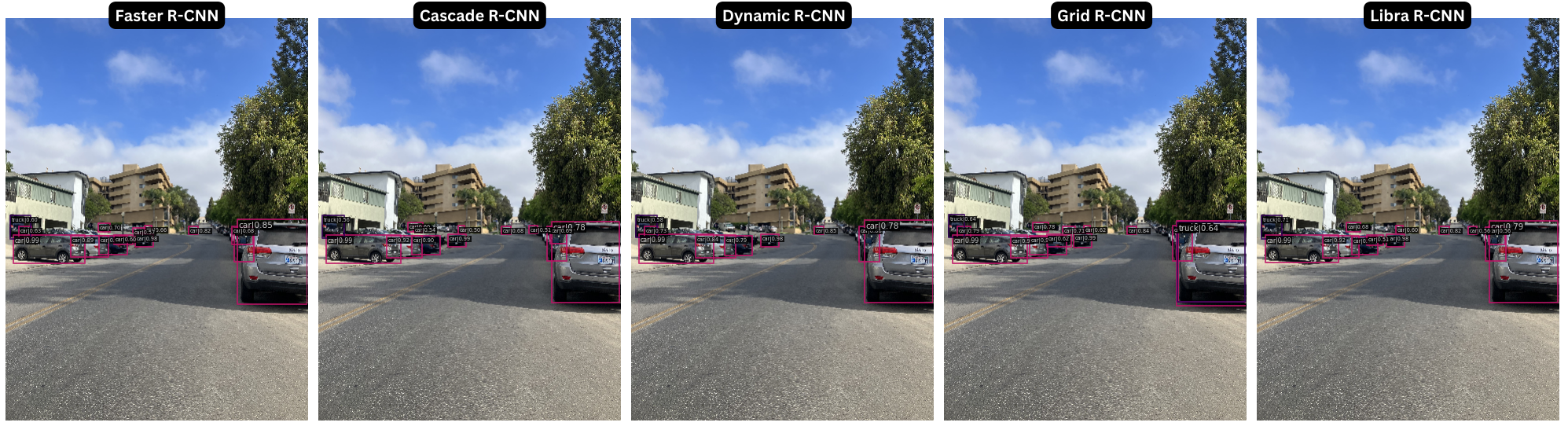
Figure 18

It is amazing that the models are able to detect the individual cars in Figure 18 above, despite their high degree of overlap. There are many cars in a line, barely visible, yet the algorithms are able to identify these cars. This shows the robustness of the models for the car class. They have learnt to detect various sections of the car, from various angles. The car training data in COCO must be very varied, helping the model perform well here. The class wise AP for the car class performance of the models ranges from 0.42 to 0.45, which means the car class has above average performance. This is clearly reflected in all the detection results we showed so far.

Method

Datasets

Our target task is object detection on the Aerial Maritime dataset, which we found publicly available on Roboflow [21]. Our source task is object detection on COCO Dataset, therefore we use models pretrained on the COCO dataset (2017 version), which is an object detection dataset with 80 classes and over 200,000 images [22].

The Aerial Maritime dataset contains bird’s eye viewpoint photos of maritime areas. It has 6 classes, which are dock, boat, lift, jetski, and car, and the superclass moveable-object, however we will only consider the 5 classes (excluding the superclass) in our analysis. We thought this data would be interesting to do transfer learning on because only 2 of the classes, namely, boat and car, are part of the COCO dataset’s 80 classes, so some new objects would need to be learned.

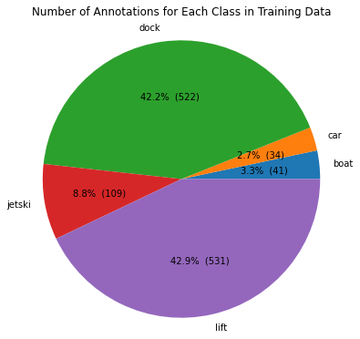
Figure 19. Number of Annotations per Class in Training Data

Exploring the training data, we can see that the dock and lift classes have the most annotations as seen in Figure 19. The train dataset has a total of 522 bounding boxes for dock and 531 for lift, making up 85% of the 1237 bounding boxes in the train dataset. This class imbalance will be useful to consider when analyzing our results.

Evaluation Metric

We chose to report the COCO Average Precision (AP) evaluation metric that is the average AP across IoU thresholds, each 0.05 apart, from 0.5 to 0.95, reported as “Average Precision (AP) @[ IoU=0.50:0.95 | area= all | maxDets=100 ]” in the MMDetection output.

Using MMDetection for Transfer Learning

OpenMMLab’s MMDetection is an open-source toolbox based on PyTorch, which allows you to build object detection models, using provided modules and APIs that can be customized [23]. MMDetection provides config files and checkpoints, or saved model weights, for certain models, pretrained on COCO dataset (2017). The config files specify everything about the model, including the model type, backbone, neck, dataset, training schedule, evaluation settings, path to checkpoint file to load pretrained weights from, and more [24]. The general definitions of backbone, neck, and head are as follows:

• backbone: the network used for feature extraction, for example, a ResNet can be used to get a feature map from the inputs
• neck: layers between the backbone and head that enhance the multi-scale features
• head: predicts the final object labels and bounding boxes to be output, using classification and regression components

The 5 models we chose to use, Faster R-CNN, Cascade R-CNN, Dynamic R-CNN, Grid R-CNN, and Libra R-CNN, had configs and pretrained weights available. We selected only object detection models, not including segmentation models, which is why we didn’t choose to use Mask R-CNN. For all the models, we used a ResNet-50 backbone and a Feature Pyramid Network (FPN) neck pretrained on the COCO dataset for 12 epochs, with the exception of the Grid R-CNN model which was pretrained for 24 epochs instead. Also, Grid R-CNN has a Group Norm (GN) head whereas the others don’t use Group Norm. In general, we tried to keep consistent settings for the various models’ configs so that the comparison would be fair. We collected various train and test metrics in order to analyze the 5 models and better understand the differences between these five variations of R-CNN.

We based our config files on these provided config files:

• configs/faster_rcnn/faster_rcnn_r50_fpn_1x_coco.py
• configs/cascade_rcnn/cascade_rcnn_r50_fpn_1x_coco.py
• configs/dynamic_rcnn/dynamic_rcnn_r50_fpn_1x_coco.py
• configs/grid_rcnn/grid_rcnn_r50_fpn_gn-head_2x_coco.py
• configs/libra_rcnn/libra_faster_rcnn_r50_fpn_1x_coco.py

We inherited the provided configs for each model, but modified the dataset from COCO to Aerial Maritime, modified the model to output one of Aerial Maritime’s 6 classes instead of COCO’s 80 classes, and added the checkpoint path to load initial weights from.

We therefore wrote 5 config files, which can be found in the DLCV-project/configs folder. Let us explain the main parts of the code in our Faster R-CNN config. We used this tutorial [25] to understand how to customize the dataset being used.

_base_ = './faster_rcnn_r50_fpn_1x_coco.py'

This line means to inherit from the faster_rcnn_r50_fpn_1x_coco.py base config.

dataset_type = 'CocoDataset'
classes = ('movable-objects', 'boat', 'car', 'dock', 'jetski', 'lift')

data_root = './data/aerial-maritime/'

data = dict(
    samples_per_gpu=2,
    workers_per_gpu=2,
    train=dict(
        type=dataset_type,
        classes=classes,
        ann_file='_annotations.coco.json',
        img_prefix='', # data_root+"train/",
        data_root="./data/aerial-maritime/train"),
    val=dict(
        type=dataset_type,
        classes=classes,
        ann_file='_annotations.coco.json',
        img_prefix='', # data_root+"valid/",
        data_root="./data/aerial-maritime/valid"),
    test=dict(
        type=dataset_type,
        classes=classes,
        ann_file='_annotations.coco.json',
        img_prefix='', # data_root+"test/",
        data_root="./data/aerial-maritime/test"))

These lines set the dataset type to COCO since our Aerial Maritime dataset is stored in the COCO data format. It changes the dataset classes to the 6 classes of the Aerial Maritime dataset, and changes the data paths to the appropriate folders where the Aerial Maritime data is stored in our project.

model = dict(
    roi_head=dict(
        bbox_head=dict(
            num_classes=6)))

The above line changes the RoI head to predict 6 classes instead of the preexisting setting of 80 classes for COCO.

load_from = 'checkpoints/faster_rcnn_r50_fpn_1x_coco_20200130-047c8118.pth'

This line tells which model checkpoints to load (pretrained weights). These are the weights after the models were trained on the COCO (source) dataset, provided by MMDetection.

work_dir = './output_dirs/faster'

The above line sets up a directory where the weights and logs will be stored during training. The folder is created in the temporary runtime in Google Colab when the notebook is running.

optimizer = dict(lr = 0.02 / 8)

The original learning rate is meant for training with 8 GPUs, but we are only using 1 GPU so we must divide it by 8.

runner = dict(max_epochs=12)

This line ensures that the training will be for 12 epochs.

evaluation = dict(metric='bbox', interval=1)

This line ensures that the bounding-box prediction metric, or mAP, will be used.

checkpoint_config = dict(interval=1)

# Set seed thus the results are more reproducible
seed = 0
# set_random_seed(0, deterministic=False)
device = 'cuda'
gpu_ids = range(1)

# We can also use tensorboard to log the training process
log_config = dict(interval = 50, hooks = [
    dict(type='TextLoggerHook'),
    dict(type='TensorboardLoggerHook')])

These lines set how often checkpoints will be saved, how often logs will be updated, and sets seeds, and device=cuda enables training on GPU.

Model Training

We decided to train the models (do finetuning on the new, Aerial Maritime dataset) for 12 epochs so that they would have sufficient time to learn from the training data. We saved the checkpoints (weights) for the models after 12 epochs and at their best epoch in the ‘weights’ folder in our project folder so that we could load these models and run tests without having to run the time-consuming training again. When running our code in our colab notebook ‘Transfer_Learning_on_Aerial_Maritime.ipynb’, we highly recommended that you do not run the Train sections and instead use the Results sections where we have code for loading the saved weights.

Links to Our Code

The Google Drive folder DLCV-project contains configs, checkpoints, data, and all code and results in the Google Colab notebooks.

The main notebook is Transfer Learning on Aerial Maritime, which contains all of our transfer learning code, results, plots, and images.

The other notebook is Evaluating Existing Models on Coco, which contains all the code related to testing the models on COCO Dataset and inference on the UCLA images, before we began any transfer learning.

To run the code, copy the DLCV-project folder to your local Google Drive. Then, make sure to change the project_path variable in the .ipynb files to the path to the DLCV-project folder in your Google Drive. Currently, it should be (project_path = ‘/content/drive/MyDrive/DLCV-project/’), which may be different from where you upload the DLCV-project folder in your Google Drive. When running our code in our colab notebook ‘Transfer_Learning_on_Aerial_Maritime.ipynb’, we highly recommended that you do not run the Train sections under each model, and instead only run the Results sections where we have code for loading the saved weights from the 12th epoch. This is because the training takes around 30 minutes per model, and saving one checkpoints file takes another 30 minutes, at least.

Results and Discussion

Training accuracy

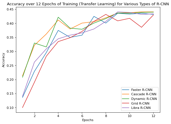
Figure 20. Accuracy over 12 epochs of training

As shown in Figure 20 above, the training accuracy over epochs follows a similar curve for all of the models, however, there are some notable differences. First, it appears that Dynamic and Cascade R-CNN learned much quicker than Faster, Libra, and Grid R-CNN. After the 4th epoch, Dynamic and Cascade R-CNN have accuracy above 0.40, while the other models do not. From epochs 5 to 8, Dynamic and Cascade R-CNN improve with a relatively lower slope than the other models, further demonstrating that Faster, Grid, and Libra learn slower than Dynamic and Cascade R-CNN.

Dynamic R-CNN uses dynamic label assignment which is adaptively assigning labels to each object proposal based on it similarity to the ground-truth objects in the image. This improves the quality of the training data and reduces the impact of mislabeled examples. Due to dynamic label assignment, the model optimizes better within one epoch. The model also uses dynamic loss which reduces the impact of bad predictions. Cascade R-CNN learns faster than the other models due to its multi-stage architecture. In one epoch, it runs through multiple detectors which explains why the accuracy increased faster in the first few epochs.

Training time

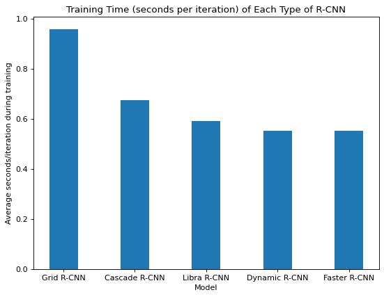
Figure 21. Training time for each type of R-CNN

Figure 21 above shows the average seconds taken per iteration (there are many iterations within an epoch) during training for each type of R-CNN, all trained with the same GPU resources. Faster R-CNN appears to require the least amount of time to train, perhaps because it is the least complex of all the models. The other models add advancements to Faster R-CNN, making them take longer to train. Most significantly, Grid R-CNN is much slower to train than the others. Due to the grid approach, more filters are required to distinguish the feature maps of different points. The additional features are used to extract features individually, then fused to obtain fusion feature maps. More convolutional layers are needed, contributing to the slower training rate.

Inference Time

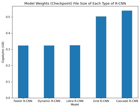
Figure 22. Inference Time for Each Type of R-CNN

Figure 22 shows the time taken for inference during testing of each R-CNN on the Aerial Maritime test data, in units of task/second, also called frames per second. Faster R-CNN appears to be the slowest, while the other models make improvements on inference time. Grid R-CNN and Cascade R-CNN are the fastest at inference time, based on our tests.

Model weights size comparison

Figure 23. Model weights file size of each type of R-CNN

Based on the checkpoint file sizes we observed for each model, there are many more model parameters for Grid and Cascade R-CNN than the other three models as shown in Figure 23. Grid R-CNN uses additional convolutional layers for the fusion feature map steps and the convolutional layers require more parameters. Cascade R-CNN trains a sequence of detectors that each require more parameters as opposed to the single detector used by the other models.

Test accuracy results

Classwise AP and mAP

Figure 24 below summarizes all the test results, showing both classwise AP and overall mAP, for each model. Certain things stand out- for example, the car class has a very high AP, and Grid R-CNN generally performs worse while Cascade and Libra R-CNN generally perform better. We will analyze the test results in detail with smaller charts that are more manageable to analyze. Figure 24 is just to give a full overview of the test results.

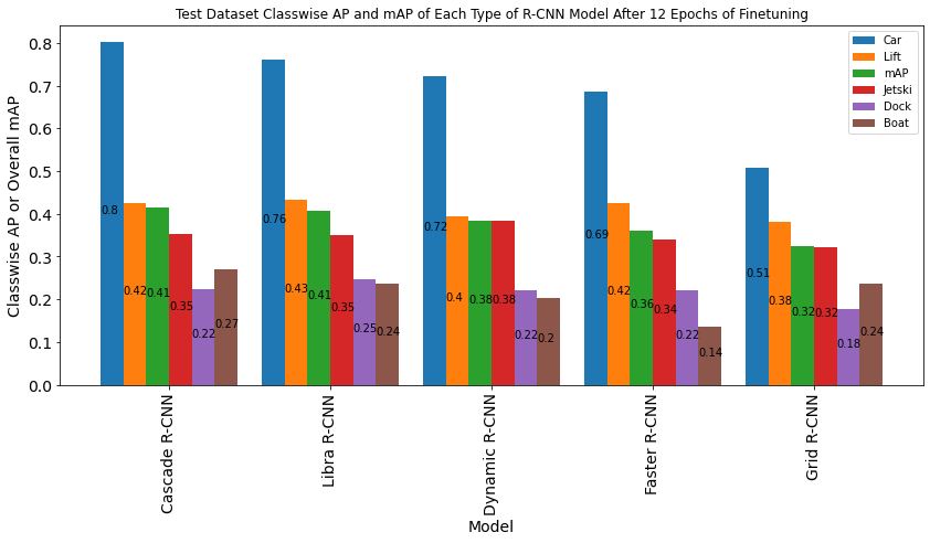
Figure 24. Test Dataset classwise AP and mAP of each type of R-CNN

mAP of each model on test set

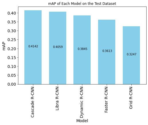
Figure 25. Test mAP of each model

Figure 25 above shows the mAP result of each model tested on the Aerial Maritime’s test split, after finetuning for 12 epochs on the Aerial Maritime train data. Cascade R-CNN had the highest mAP of 0.41. We would expect Faster R-CNN to be the worst performing model, since all other models have enhancements that are supposed to improve Faster R-CNN. Our results are mostly consistent with our expectations. Dynamic, Libra, and Cascade R-CNN all performed better than Faster R-CNN by 2.32, 4.46, and 5.29 percentage points respectively. This only unusual result is that Grid R-CNN performed worse than Faster R-CNN after transfer learning. This may be due to the extreme imbalance between the training data classes. Grid R-CNN supposedly performs better when objects are densely packed together or partially occluded, but the objects in our dataset are more spreadout and large, rendering that attribute less effective. Grid R-CNN also uses feature fusion, generating sets of multi-scale feature maps that may be unnecessary for our model. The small dataset size might also mean that such a big/complex model like Grid R-CNN is not bound to perform well. Grid R-CNN uses a CNN to determine the bounding boxes, whereas the other models use FC layers to find the bounding boxes, making Grid R-CNN fundamentally different from the rest.

Comparing classes, average classwise AP and mAP

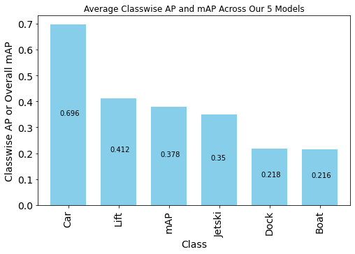
Figure 26. Average classwise AP and mAP across models

Figure 26 above shows the classwise AP averaged across our 5 models, and the average mAP for reference as well. The two classes that were already in the COCO dataset, car and boat, have very different results. The car class had the best performance across all models, even though only 2.7% of train data annotations were labeled car. This could be because we saw that the pretrained models from COCO were already quite good at detecting cars. The car class AP was between 0.42 to 0.45 for all the models, when tested on COCO. After finetuning for 12 epochs on Aerial Maritime dataset, the average car class AP is 0.696. Assuming the train data was representative of the test data, we can infer that the test data had few car images, so there was less chance for the model to make a mistake on them, leading to a high car class AP. The boat class AP is poor in comparison to car. This is surprising because boat is one of COCO’s 80 classes. However, the boats look very different from the aerial viewpoint compared to ground-level view. The COCO boat images are likely all from the ground-level view so the learned properties of boats might not be transferable to aerial view. The boat dataset also had few training examples in the Aerial Maritime dataset which we would expect causes poor performance for that class. The model performs well for classifying lift with 0.412 average AP, while it does relatively poorly for dock with 0.218 average AP. A possible reason why lift was predicted well is that shiplifts are similar looking to some of the objects in the COCO Dataset’s 80 classes, so the pretrained models had information in their weights that could transfer to this task. Another possibility is that shiplifts are generally similar looking to each other, and less variance in how they look makes them easier to learn. Also, docks and jetski may have more complex shapes and shading, as docks have many wood panels, and jet skis are oddly shaped, making them harder to learn.

Sample predictions on images

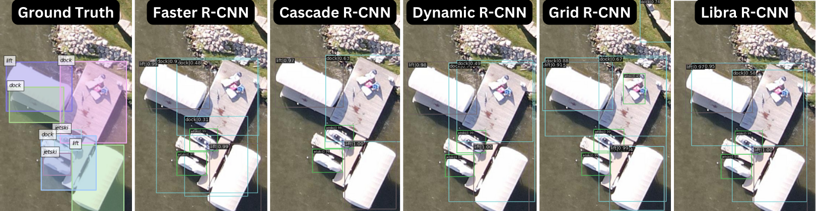
Figure 27. A selected test image.

For Figure 27, in the ground truth image, there are 2 lifts, 3 docks, and 2 jetskis. This image has various objects close together with overlapping bounding boxes. Faster R-CNN correctly detects both jetskis, both lifts, but has trouble locating the dock objects with confidence. There are overlapping dock bounding boxes with low confidence values. A large box identifying the dock is used rather than 3 like in the ground truth image. The 3 docks are connected so this may be why Faster R-CNN recognized all three as one object. Cascade R-CNN was able to correctly identify everything except for the 2 smaller docks. The main dock that it recognized did not have a high confidence value either, indicating that this model had some trouble identifying this class in general. Dynamic R-CNN found 2 overlapping bounding boxes indicating ‘dock’ which is strange since only one bounding box should have been identified. The confidence value is also lower with those two bounding boxes. Grid R-CNN incorrectly identifies a non-dock object in the corner as a dock with relatively high confidence, and multiple overlapping boxes were found for the dock areas. Libra R-CNN manages to include all the docks within bounding boxes, but with incorrect localizations. Overall, all the models correctly identified the lifts and jetskis but had trouble localizing the docks. The docks are rectangular and are slightly askew in this image which probably made it difficult to localize it correctly on top of being connected to each other.

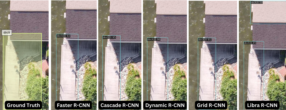
Figure 28. A selected test image.

For Figure 28, the ground truth image has a bounding box identifying a dock that includes an asymmetrical area on the end. All 5 models correctly identify the dock but fail to include the asymmetrical area. This may have to do with the docks present in the training data and how many of them are simple rectangles.

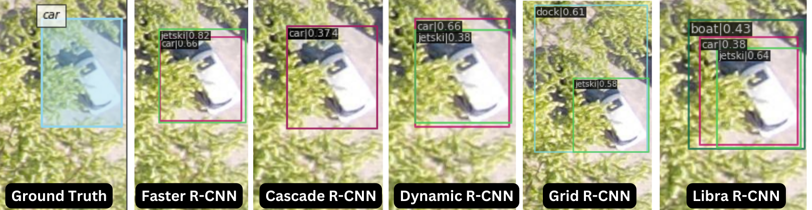
Figure 29. A selected test image.

For Figure 29, only a car is identified in the ground truth image. However, Faster, Dynamic, Grid, and Libra R-CNN all identified other objects that were incorrect. Faster, Dynamic, and Grid incorrectly identified the object as jetski. Grid drew two bounding boxes for the object but both labels were incorrect. Libra drew three bounding boxes, identifying the object ask boat, car, and jetski. These 3 objects have some similar features which may be the reason for the poor performance. After inspecting the training data, we find that there is a large class imbalance. Jetski, boat, and car are highly underrepresented, with car having the least amount of samples in the training dataset. This would be a more plausible explanation for the poor performance from the models.

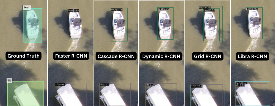
Figure 30. A selected test image.

All the models correctly identified the boat and lift in Figure 30. The boat has distinct features and is not directly next to any other objects which lead to the high accuracy. Grid R-CNN drew two bounding boxes for the boat, with one of them having a very low confidence rate. This is a strange outcome as Grid R-CNN uses NMS (non-maximum suppression) and should only display one of these bounding boxes. Libra and Grid R-CNN also identified the lift as a dock, which may be due to the fact that the object is only partially visible. Overall, since the objects are quite separated in the image, the models performed well.

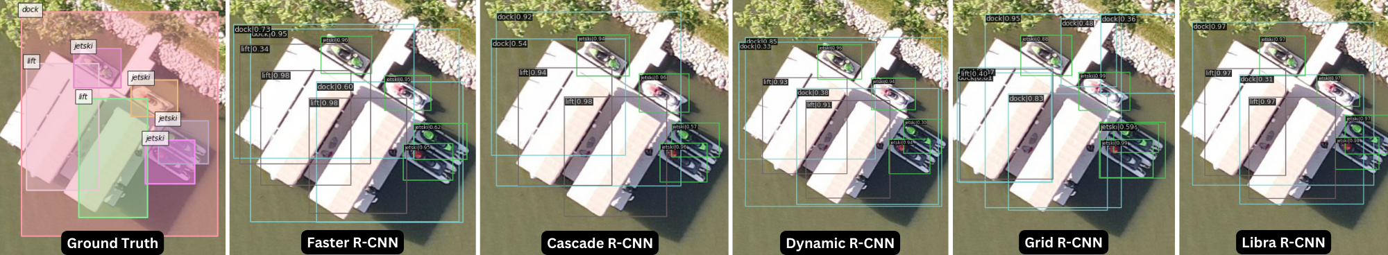
Figure 31. A selected test image.

In Figure 31, there should be 4 jetskis, 2 lifts, and 1 dock identified with bounding boxes. All of the models accurately identify the 4 jetskis and 2 lifts, but each model interpreted the dock differently. Multiple bounding boxes for the dock were produced. This is most likely due to the fact that the lifts are very close to the dock, segmenting the dock so that it appears there are more than 1 dock location. The ground truth bounding box for dock overlaps with all the other objects in the image so that might also be problematic for this specific image.

Adversarial attacks

We tested the robustness of the various R-CNN models after finetuning on the new dataset by testing images with adversarial attacks. An adversarial attack refers to changing the image in some way to prevent the algorithm from correctly detecting objects. Often, images are perturbed with noise in clever ways to have them appear to the algorithm as a different object entirely. In this case, we changed some pixels of the image to black (R, G, B = 0, 0, 0) and saw the impact on predictions. We used a variety of locations and sizes for the patches. The figures below show the results of the 5 models on the Aerial Maritime images with adversarial attacks. For reference, the predictions of each model run on the test image before any adversarial attack are shown below in Figure 32. Each of the models correctly identifies the dock, lift, and jetski where there is no adversarial attack.

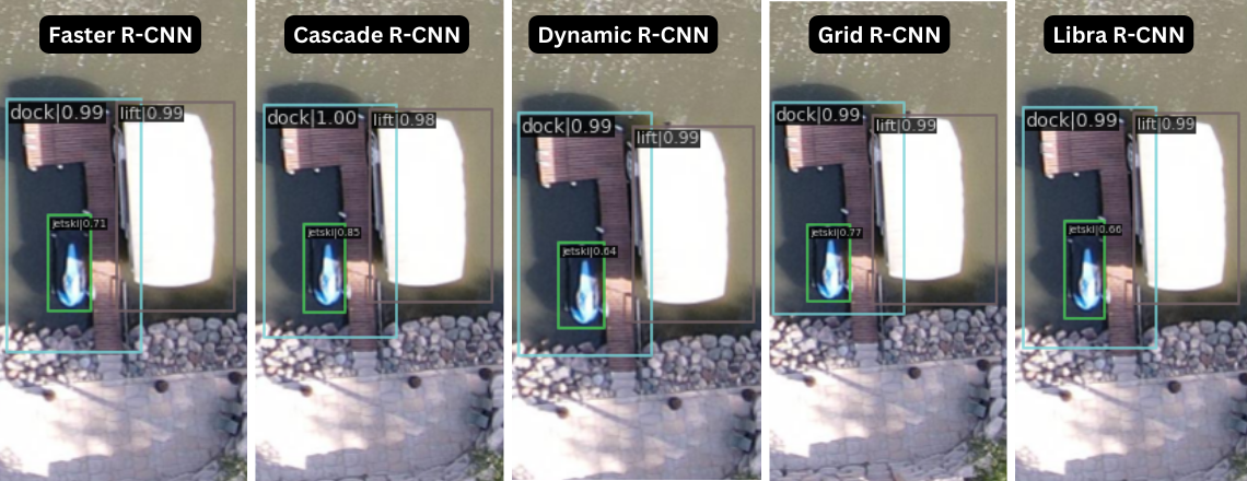
Figure 32. Predictions of Each Model on the Image, Before Any Adversarial Attack.

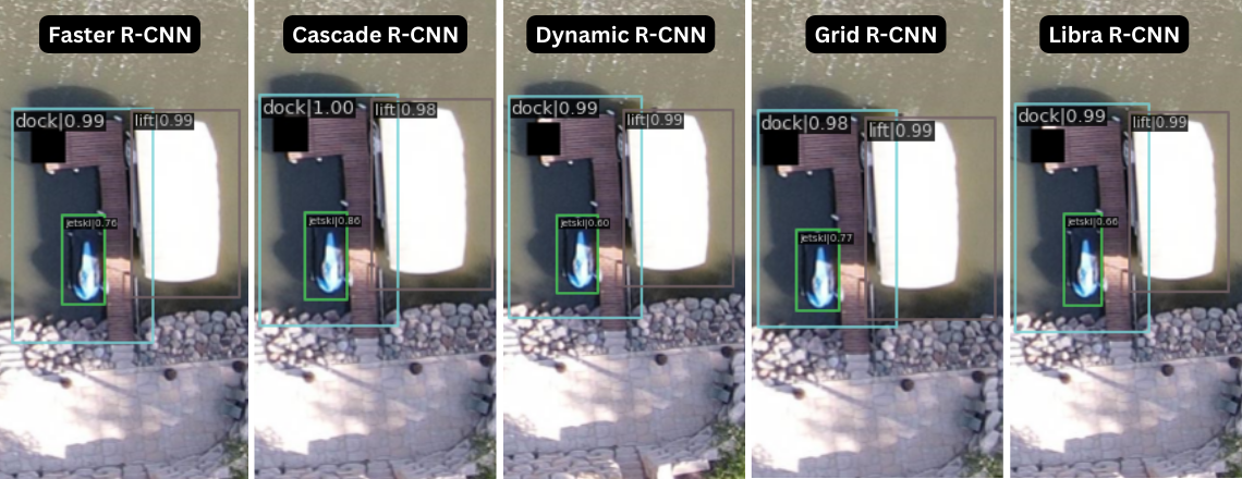
Figure 33. One small black box.

For the first adversarial attack in Figure 33, we blocked the pixels in the top left area of the dock. This was a test to explore the effect on the dock identification. Since only a small part of the dock was hidden, all the models correctly identified and localized the dock object with very high confidence. The other objects in the image were left untouched and consequently had no change in prediction outcomes.

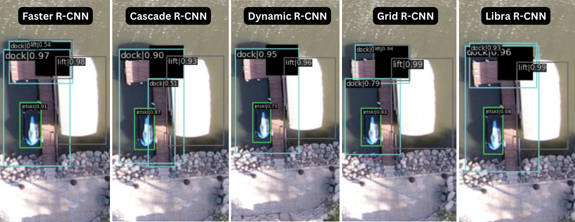
Figure 34. One medium-sized black box.

The second adversarial attack in Figure 34 blocked parts of both the dock and lift with a larger box. Faster and Grid R-CNN drew a bounding box around the black box and identified it as a lift although it was not meant to be an object. The lift was correctly identified with high confidence values by all the models even though part of it was obscured. Multiple bounding boxes were identified for the dock by Cascade, Grid, Libra and Faster, likely due to the black box seemingly splitting the dock into two. Surprisingly, the bounding boxes from Dynamic R-CNN had no decrease in accuracy, only with a slightly lower confidence level.

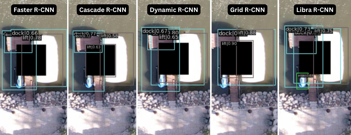
Figure 35. One large black box.

For the third adversarial attack in Figure 35, we used a larger box to partially obscure all the objects in the image. Only Libra R-CNN was able to identify the jetski. Grid R-CNN once again incorrectly identified the black box as a lift. Overall, all the models had trouble identifying the dock and drew multiple bounding boxes as the block box had divided it into 2 parts. The models also identified the lift with lower confidence levels.

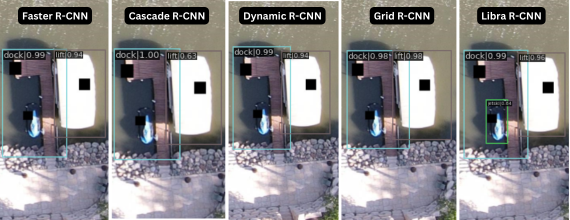
Figure 36. Three small black boxes.

The fourth adversarial attack in Figure 36 included small black boxes obscuring part of each object present. Once again, only Libra R-CNN was able to identify the jetski. The other models were not able to locate or identify it all even though only a small part of the jetski was obscured. The lift was correctly identified in all the models, although Cascade R-CNN identified it with much lower confidence than before. The dock results were described in the first adversarial attack discussion.

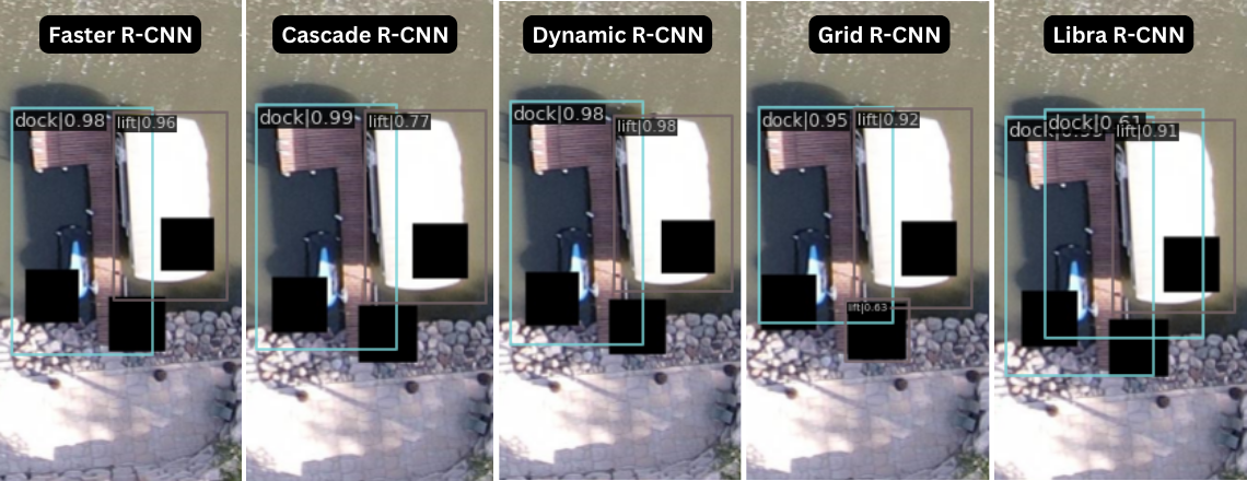
Figure 37. Three large black boxes.

The fifth adversarial attack in Figure 37 included larger boxes covering all three objects. None of the models were able to identify the jetski. This is likely because part of the head of the jetski was hidden, and the head had a lot of unique features to the jetski class. The dock was correctly identified by all the models as the black box was covering a far corner of the object that did not interfere as much as some of the previous adversarial attacks. The lift was also consistently identified correctly. Libra R-CNN did have a second bounding box identifying ‘dock’, which is strange since there was already an overlapping dock identified.

Overall, the models struggled with identifying the jetski class the most, likely due to its smaller scale. The lift was identified the most accurately across the models, probably due to its relatively large size, simple features, and uniform shape. The dock was mostly identified correctly but adversarial attacks covering part of the dock lead to incorrect localization of the object. The large variation of dock shapes probably increased the models’ ability to identify it but since most of the docks are very close to other objects and may suffer from occlusion, the localization performance of the docks was less strong. From these experiments, we can deduce that Libra R-CNN identifies smaller objects better than the other models, while Dynamic R-CNN performed the best when parts of objects were obscured. Cascade, Grid, and Faster R-CNN performed worse and struggled with the correct localization of the dock.

Conclusion

By using a new dataset, we explored the transfer learning performance of 5 R-CNN based object detection models: Faster R-CNN, Cascade R-CNN, Dynamic R-CNN, Grid R-CNN, and Libra R-CNN. In the training stage, Dynamic and Faster R-CNN were the fastest to train and Grid R-CNN was the slowest to train. The training accuracy scores for all the models were similar after 12 epochs at around 0.45, but Cascade and Dynamic R-CNN learned faster in the first few epochs. This is because Cascade R-CNN uses a sequence of detectors trained with increasing IoU thresholds, and Dynamic R-CNN dynamically adjusts IoU Threshold for label assignment and the shape of regression loss function during training, both changes that can easily be seen in a short duration of time. Libra R-CNN’s strategies to combat imbalance helped it achieve a high mAP as well, it just took slightly longer to show its strength. Cascade, Libra, and Dynamic R-CNN performed better than Faster R-CNN on the test data as hypothesized but we found that Grid R-CNN actually performed worse. This is surprising as it is a variant of Faster R-CNN that attempts to improve on Faster R-CNN’s performance. However, the dataset we selected had a lot of flaws that Grid R-CNN struggled with. We felt that this could be because Grid R-CNN is very different from the others with its grid-guided localization approach. Also, it could be because our dataset was small and imbalanced, with certain classes being very underrepresented. The object classes also had varying scale in the images, which also made identifying certain objects more challenging. The models that made improvements to mitigate class imbalance and problems of scale proved to perform better on our dataset, such as Libra R-CNN and Cascade R-CNN. Across the object classes, the 5 models identified ‘car’ the best and ‘boat’ and ‘dock’ the worst. The COCO dataset likely had different representations of these classes compared to our aerial dataset, which is probably why the performance was weaker. We performed adversarial attacks to test the robustness of the models, and found Libra R-CNN and Dynamic R-CNN to perform the best. Other ways that transfer learning could have been explored but were not implemented include varying sample sizes, freezing specific layers, using different pretrained datasets, and changing pretrained weights. We did not choose to perform these experiments due to the limitations of our selected dataset and the model configurations provided by MMDetection although they are worthwhile to explore in the future.

Video Presentation

The video presentation is linked here.

Reference

[1] ImageNet Large Scale Visual Recognition Challenge 2017 (ILSVRC2017). https://www.image-net.org/challenges/LSVRC/2017/index.php

[2] Zou, Z., Chen, K., Shi, Z., Guo, Y., & Ye, J. (2023). Object detection in 20 years: A survey. Proceedings of the IEEE.

[3] Viola, P., & Jones, M. (2001, December). Rapid object detection using a boosted cascade of simple features. In Proceedings of the 2001 IEEE computer society conference on computer vision and pattern recognition. CVPR 2001 (Vol. 1, pp. I-I). Ieee.

[4] Lowe, D. G. (2004). Distinctive image features from scale-invariant keypoints. International journal of computer vision, 60, 91-110.

[5] Dalal, N., & Triggs, B. (2005, June). Histograms of oriented gradients for human detection. In 2005 IEEE computer society conference on computer vision and pattern recognition (CVPR’05) (Vol. 1, pp. 886-893). Ieee.

[6] Krizhevsky, A., Sutskever, I., & Hinton, G. E. (2017). Imagenet classification with deep convolutional neural networks. Communications of the ACM, 60(6), 84-90.

[7] Girshick, R., Donahue, J., Darrell, T., & Malik, J. (2014). Rich feature hierarchies for accurate object detection and semantic segmentation. In Proceedings of the IEEE conference on computer vision and pattern recognition (pp. 580-587).

[8] Girshick, R. (2015). Fast r-cnn. In Proceedings of the IEEE international conference on computer vision (pp. 1440-1448).

[9] Ren, S., He, K., Girshick, R., & Sun, J. (2015). Faster r-cnn: Towards real-time object detection with region proposal networks. Advances in neural information processing systems, 28.

[10] Redmon, J., Divvala, S., Girshick, R., & Farhadi, A. (2016). You only look once: Unified, real-time object detection. In Proceedings of the IEEE conference on computer vision and pattern recognition (pp. 779-788).

[11] Liu, W., Anguelov, D., Erhan, D., Szegedy, C., Reed, S., Fu, C. Y., & Berg, A. C. (2016). Ssd: Single shot multibox detector. In Computer Vision–ECCV 2016: 14th European Conference, Amsterdam, The Netherlands, October 11–14, 2016, Proceedings, Part I 14 (pp. 21-37). Springer International Publishing.

[12] Lin, T. Y., Dollár, P., Girshick, R., He, K., Hariharan, B., & Belongie, S. (2017). Feature pyramid networks for object detection. In Proceedings of the IEEE conference on computer vision and pattern recognition (pp. 2117-2125).

[13] Carion, N., Massa, F., Synnaeve, G., Usunier, N., Kirillov, A., & Zagoruyko, S. (2020). End-to-end object detection with transformers. In Computer Vision–ECCV 2020: 16th European Conference, Glasgow, UK, August 23–28, 2020, Proceedings, Part I 16 (pp. 213-229). Springer International Publishing.

[14] Kukil. (2022) Intersection over Union (IoU) in Object Detection & Segmentation. https://learnopencv.com/intersection-over-union-iou-in-object-detection-and-segmentation/

[15] Kundu, R. (2023). YOLO: Algorithm for Object Detection Explained. https://www.v7labs.com/blog/yolo-object-detection#h3

[16] Wang, C. Y., Bochkovskiy, A., & Liao, H. Y. M. (2022). YOLOv7: Trainable bag-of-freebies sets new state-of-the-art for real-time object detectors. arXiv preprint arXiv:2207.02696.

[17] Cai, Z., & Vasconcelos, N. (2018). Cascade r-cnn: Delving into high quality object detection. In Proceedings of the IEEE conference on computer vision and pattern recognition (pp. 6154-6162).

[18] Zhang, H., Chang, H., Ma, B., Wang, N., & Chen, X. (2020). Dynamic R-CNN: Towards high quality object detection via dynamic training. In Computer Vision–ECCV 2020: 16th European Conference, Glasgow, UK, August 23–28, 2020, Proceedings, Part XV 16 (pp. 260-275). Springer International Publishing.

[19] Pang, J., Chen, K., Shi, J., Feng, H., Ouyang, W., & Lin, D. (2019). Libra r-cnn: Towards balanced learning for object detection. In Proceedings of the IEEE/CVF conference on computer vision and pattern recognition (pp. 821-830).

[20] Lu, X., Li, B., Yue, Y., Li, Q., & Yan, J. (2019). Grid r-cnn. In Proceedings of the IEEE/CVF Conference on Computer Vision and Pattern Recognition (pp. 7363-7372).

[21] Solawetz, J. (2020) Aerial Maritime Drone Dataset. MIT. https://public.roboflow.com/object-detection/aerial-maritime

[22] COCO 2017 Object Detection Task. https://cocodataset.org/#detection-2017

[23] MMDetection GitHub. https://github.com/open-mmlab/mmdetection

[24] MMDetection: Tutorial 1: Learn About Configs. https://mmdetection.readthedocs.io/en/latest/tutorials/config.html

[25] MMDetection: Tutorial 2: Customize Datasets. https://mmdetection.readthedocs.io/en/latest/tutorials/customize_dataset.html