Skin Lesion Classification
It is crucial to catch skin cancer at an early stage. This can be done using image classification techniques. Specifically, this post aims to explore using different methods to handle class imbalance while classifying skin lesions using the HAM10000 dataset.

Abstract
I built a model for skin lesion classification trained and evaluated on the HAM10000 dataset. To deal with the high class imbalance in the dataset, various methods were employed, including a hierarchy of classifiers as well as data augmentation and repeats. In the end, a model ensemble was built of different hierarchical classifiers, where each hierarchical classifier contained 4 convolutional neural networks that were built using pre-trained versions of AlexNet, VGG, EfficientNet (B4), and ResNet-18. In addition, four of these hierarchical classifiers were built with additional access to metadata contained in the dataset. This hierarchical classifier structure was able to achieve better results on unseen data when compared to a non-hierarchical structure. Multiple different ensembles of these hierarchical classifiers were tested out, with the best choice being that of the four models given access to metadata, achieving an accuracy of 67.5%.
Introduction
Skin cancer can be extremely dangerous, but is usually harmless unless it isn’t caught until a later stage, once it has already advanced past the skin alone and into other parts of the body. Because of this, it is crucial to catch it early. With deep learning, it is possible to classify various skin lesions as cancerous or not, which is highly beneficial as this can prevent a doctor’s visit (if accurate enough), which would allow for more accessibility. In this project, the goal is to try and build the best model possible using the given resources. In particular, it will explore the building of a model ensemble using various techniques to deal with the class imbalance seen in the dataset.
Method
Dataset
The dataset that I have chosen to work with throughout the course of this project is the HAM10000 dataset, which is short for “Human Against Machine with 10000 training images”. It is a dataset developed by Harvard Dataverse with 10015 dermascopic training images along with associated metadata. The labels on the data consist of the following skin lesion types with the associated number of images in each class:
- Acitinic keratoses and intraepithelial carcinoma (‘akiec’): 327
- Basal cell carcinoma (‘bcc’): 514
- Benign keratosis-like lesions (solar lentigines / seborrheic keratoses and lichen-planus like keratoses) (‘bkl’): 1099
- Dermatofibroma (‘df’): 115
- Melanoma (‘mel’): 1113
- Melanocytic nevi (‘nv’): 6705
- Vascular lesions (angiomas, angiokeratomas, pyogenic granulomas and hemorrhage) (‘vasc’): 142
Along with the images, the dataset also contains metadata for each image, including the sex of the person the image was taken of, along with the locality skin lesion (abdomen, back, etc.). This metadata was loaded in using pandas and converted to one-hot encoding.
Data Augmentation
Data augmentation is an essential aspect to prevent overfitting to the training data by creating slight variations on the data. Currently, I am using the following data transforms on the training set, which employs various PyTorch built-in functions:
train_transform = transforms.Compose([
    transforms.RandomHorizontalFlip(),
    transforms.RandomVerticalFlip(),
    transforms.RandomRotation((0, 360)),
    transforms.ColorJitter(brightness=0.1, contrast=0.1, saturation=0.1),
    transforms.Resize((128, 128)),
    transforms.ToTensor(),
    transforms.Normalize((0.485, 0.456, 0.406), (0.229, 0.224, 0.225)) # ImageNet statistics
])
Below are some visualizations of before and after the transforms:
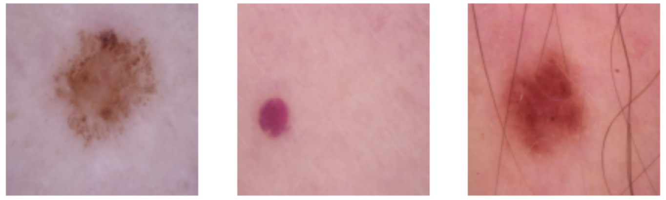
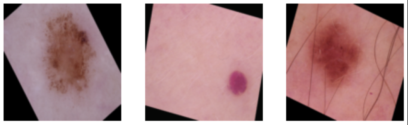
The Model
Baseline Models
All of the following baseline models were using weights from being pre-trained on ImageNet and were then finetuned to the HAM10000 dataset. The final fully-connected layers of the models are also modified to have the specified number of outputs required for each network.
AlexNet
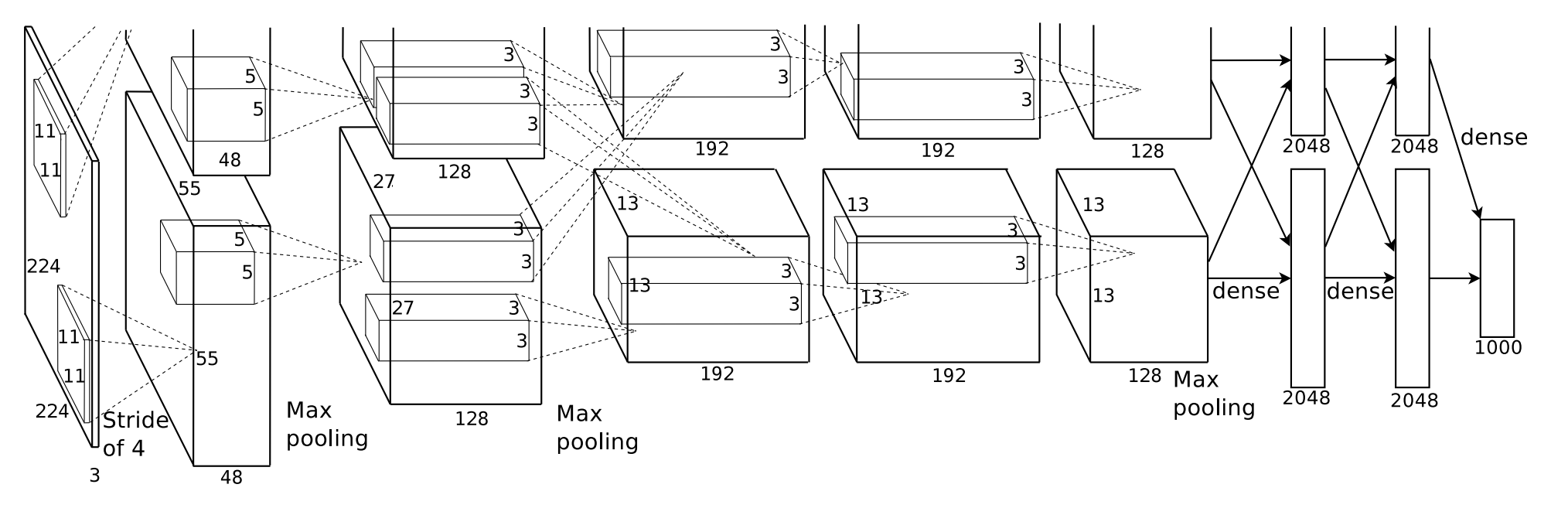
Developed primarily by Alex Krizhevsky with assistance from Ilya Sutskever and Turing Award winner Geoffrey Hinton, AlexNet was one of the first deep convolutional neural networks used for image classification. It contains 5 convolutional layers, along with 3 max pooling layers, 2 normalization layers, and 2 fully-connected layers while using ReLU as its activation function.
VGG
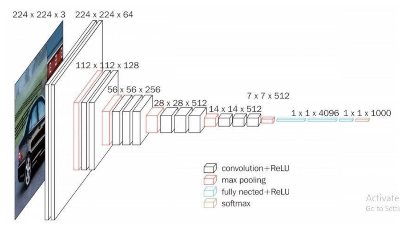
Developed by Karen Simonyan and Andrew Zisserman in 2015, VGG (short for Visual Geometry Group) is another deep convolutional neural network that s most notable for its increased depth when compared to its predecessors. The specific VGG model used in this project is VGG-16. VGG-16 consists of 13 convolutioanl layers, along with 5 max pooling layers and 3 fully-connected layers. The 16 refers to 16 total layers with weights (13 conv + 3 fc).
ResNet
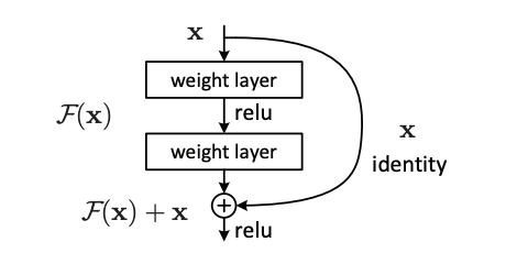
ResNet (short for residual networks) is an architecture developed by prolific computer vision researcher Kaiming He et al in 2015 that is most notable for its introduction of residual connections. These residual connections added together the previous layer’s activations to the current layer’s, solving the previously perplexing vanishing-gradient problem in computer vision. The ResNet architecture elected for use in this project is ResNet-18, which is an 18-layer neural network using residual connections.
EfficientNet
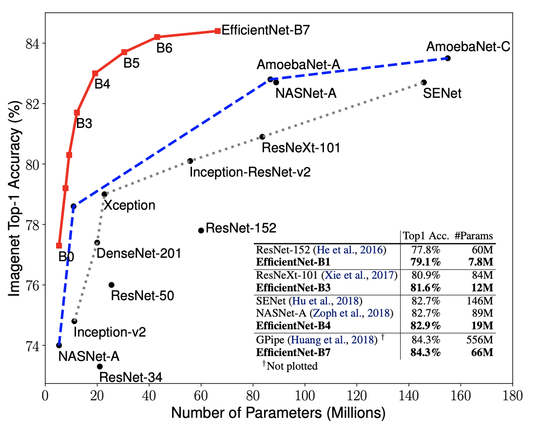
EfficientNet is a deep convolutional network architecture developed by Google in 2020 that aimed to achieve the best performing model both in accuracy and efficiency. This was done by looking into the effects of scaling a model’s depth, width, and resolution had on the efficiency and accuracy of a model. The researchers then proposed “a new scaling method that uniformly scales all dimensions of depth/width/resolution using a simple yet highly effective compound coefficient.” This scaling method was then used on various already-successful models to further improve them. The EfficientNet model that is used in this project is EfficientNet-B4, which was chosen because its position on the above curve suggests that it is a good medium of performance and efficiency.
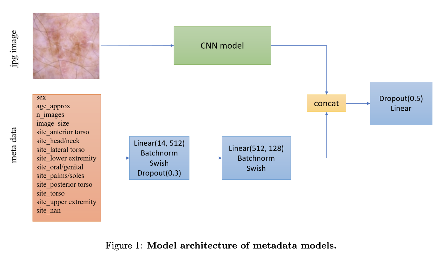
Including Metadata
Some of the models are trained using metadata. For those models, they follow the following architecture from the one used in the winning solution to the SIIM-ISIC Melanoma Classification Challenge in 2020. This includes feeding the metadata through its own neural network before concatenating the outputs from that network with the outputs from the CNN used on the image, before finally feeding this to the final fully-connected layer. The only differences from this layout and my own is the use of leaky ReLU in my implementation instead of the Swish activation function, as well as the absence of the final dropout and a slight difference in metadata (as I am using a different dataset).
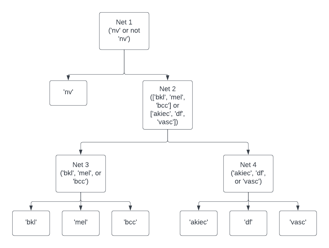
Hierarchical Classifier
To handle the immense class imbalance present in the data (as can be seen in the above section on the dataset), a hierarchical classifier approach was employed. This hierarchical classifier involved training four separate neural networks for each classifier. The first network is used to distinguish between the class ‘nv’ or not ‘nv’, the second to distinguish whether the image was one of [‘bkl’, ‘mel’, ‘bcc’] or [‘akiec’, ‘df’, ‘vasc’], and then the final two classifiers were for final classification on each of those two sets. In order to train these classifiers, the dataset was given different labels depending on which net was being trained. Another tool to further assist in handling the class imbalance was the repeat of certain images in the dataset, depending on which net was being trained, in order to try and achieve the greatest balance between classes. Specifically, ‘bcc’ and ‘vasc’ images were repeated once in the training set for the final classification networks, while ‘df’ was repeated twice in the final classification network.
Training Setup
For training, all networks used Adam as the optimizer and cosine annealling as the learning rate scheduler with cross entropy loss as the loss function. The first net (‘nv’ or not ‘nv’) had an initial learning rate of 0.1, while the rest had an initial learning rate of 0.01. The first two nets were trained for 5 epochs, while the last two (those used for final classification) were trained for 10 epochs.
Ensemble Method
Model ensembling is a great way of avoiding any biases that may be present in a single model. In this project, I ensembled 8 total different hierarchical classifiers built with the following baseline models: AlexNet, VGG-16, EfficientNet-B4, and ResNet-18 (4 with metadata, 4 without). The method used for ensembling these models was a simple average of the output logits from all of the models before final classification.
Results
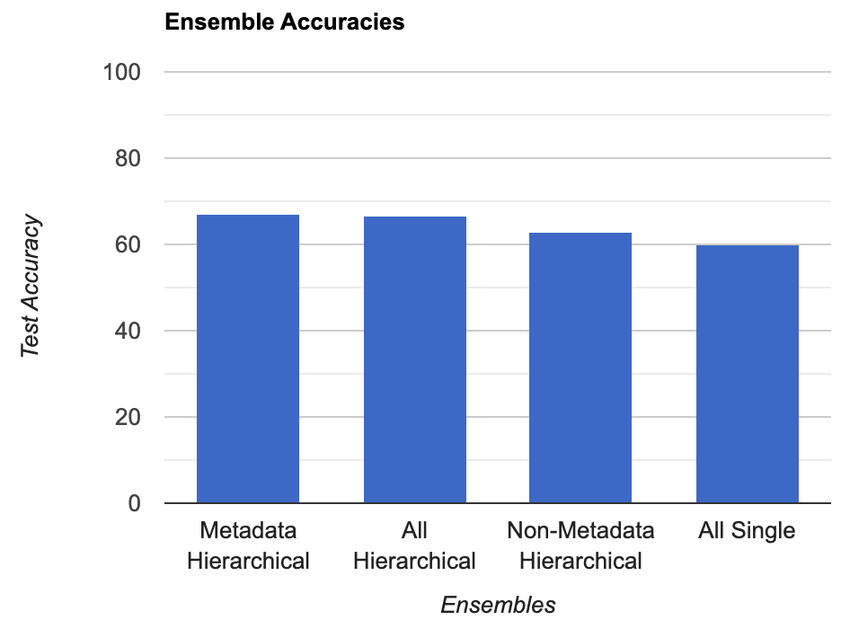
In the end, the 8 hierarchical models ensembled together were able to achieve 66.5% accuracy on unseen data. This hierarchical ensemble performed far better than a single-model ensemble, where the single model ensemble consisted of 8 models, also AlexNet, VGG-16, ResNet-18, and EfficientNet-B4, metadata and not, trained for 2 epochs, which was only able to achieve 60.09% accuracy. Furthermore, when two ensembles were created from the hierarchical classifiers, one with solely the metadata models and one with all but the metadata models, the metadata models performed better with 67.2% accuracy compared to the non-metadata ensemble’s 63.0%. In conclusion, the best model then is the hierarchical ensemble of metadata models built with AlexNet, VGG-16, ResNet-18, and EfficientNet-B4 as the backbone networks.
Discussion
The ordering of the accuracy scores from highest to lowest makes complete sense. The hierarchical structure allowed for the models to perform better on the lower volume data, as each classifier was trained on a dataset that had an even distribution of labels. As such, class imbalance had no effect. Furthermore, the increased performance of the metadata models also makes sense, as common sense says that the extra information should help with the classification task. Perhaps the only really perplexing thing about this study is how close the performance of the different model ensembles is, as I expected the hierarchical ensemble to far outperform the single-model one. One potential reason for this is the lack of training time / computing resources. It would be interesting to see if allowing for the models to train for a longer time would further increase the gap in performance.
References
- [1] Tschandl, Philipp. 2018. “The HAM10000 dataset, a large collection of multi-source dermatoscopic images of common pigmented skin lesions”. https://doi.org/10.7910/DVN/DBW86T. Harvard Dataverse.
- [2] Krizhevsky, Sutskever, Hinton. 2012. “ImageNet Classification with Deep Convolutional Neural Networks”. https://proceedings.neurips.cc/paper_files/paper/2012/file/c399862d3b9d6b76c8436e924a68c45b-Paper.pdf.
- [3] Simonyan, Zisserman. 2015. “Very Deep Convolutional Networks for Large-Scale Image Recognition”. https://arxiv.org/pdf/1409.1556.pdf.
- [4] He et al. 2015. “Deep Residual Learning for Image Recognition”. https://arxiv.org/pdf/1512.03385.pdf.
- [5] Tan, Le. 2020. “EfficientNet: Rethinking Model Scaling for Convolutional Neural Networks”. https://arxiv.org/pdf/1905.11946.pdf.
- [6] Ha, Liu, Liu. “Identifying Melanoma Images using EfficientNet Ensemble: Winning Solution to the SIIM-ISIC Melanoma Classification Challenge”. https://arxiv.org/pdf/2010.05351v1.pdf.