Trajectory Prediction

Trajectory prediction of pedestrians and vehicles involves utilizing information relating to the previous locations of such subjects to predict where they will be in the future, which is important in contexts such as that of an autonomous vehicle but may be complex as subjects may respond unpredictably in a real-time environment. We examine two approaches to trajectory prediction, a stepwise goal approach with SGNet [1] [2] and a graph approach with PGP [3] [4], while also briefly examining a third model, Trajectron++ [5] [6], as a comparison. We work with the ETH / UCY (obtained through the Trajectron++ repository [6]) and nuScenes [7] datasets during these studies.

Environment Setup

The studies were run on a Google Cloud Platform Linux virtual machine with a single GPU. To set up the environment, begin by navigating to or creating the desired project directory and running the commands

mkdir Checkpoints
mkdir Data
mkdir Models
mkdir Outputs

The project directory will be denoted as ProjectRoot, which is to be treated as an absolute filepath and is to be replaced with the actual filepath to the project directory.

Models

Stepwise Goal-Driven Networks for Trajectory Prediction

Paper: https://doi.org/10.48550/arXiv.2103.14107 [1]

Repository: https://github.com/ChuhuaW/SGNet.pytorch [2]

Overview

This paper introduces a recurrent neural network (RNN) called Stepwise Goal-Driven Network (SGNet) for predicting trajectories of observed agents (e.g. cars and pedestrians) [1].

Unlike previous research which model an agent as having a single, long-term goal, SGNet draws on research in psychology and cognitive science to model an agent as having a single, long-term intention that involves a series of goals over time [1].

To this end, SGNet estimates and uses goals at multiple time scales to predict agents’ trajectories. It comprises an encoder that captures historical information, a stepwise goal estimator that predicts successive goals into the future, and a decoder to predict future trajectory [1].

Technical Details

The model uses a recurrent encoder-decoder architecture and consists of an encoder, a stepwise goal estimator (SGE), two goal aggregators, an optional conditional variational autoencoder (CVAE) for stochastic results, and a decoder. Both the encoder and the decoder are recurrent and evolve over time [1].

The encoder encodes an agent’s movement behavior into a latent vector by embedding historical trajectory information. At each time step, the input feature is concatenated with aggregated goal information from the previous time step, then the hidden state is updated via a recurrent cell [1].

The stepwise goal estimator predicts coarse stepwise goals for use in the encoder and decoder. At each time step, the input is concatenated with predicted stepwise goals from the previous step to form the input to the encoder. The SGE also uses a goal aggregator that uses an attention mechanism to learn the importance of each stepwise goal to reduce the impact of inaccurate goals [1].

The conditional variational autoencoder learns the distribution of the future trajectory given the observed trajectory. The CVAE comprises a recognition network, a prior network, and a generation network, each of which is implemented using fully-connected layers [1].

SGNet uses root mean square error (RMSE) as the loss function. On the ETH/UCY datasets, SGNET evaluates performance using two metrics: average displacement error (ADE) and final displacement error (FDE). ADE measures the average L2 distance between the ground truth and predicted trajectories along the whole trajectory. FDE measures the L2 distance between the end points of the ground truth and predicted trajectories [1].

Setup

The following Colab notebook allows for training and testing SGNet as well as visualizing its output. The SGNet code in the GitHub repository published by the paper authors did not return trajectory data or include visualization code, so some setup and extra code is required to make the Colab notebook work.

To try out SGNet for yourself, follow the instructions in this notebook: https://colab.research.google.com/drive/16vEoKwFUdcCuMD6FKGhkLS7zPjHe7e7_?usp=share_link

Results

In the paper, the authors achieved state-of-the-art performance on ETH/UCY data based on ADE and FDE. For example, SGNet achieved ADE=0.40 and FDE=0.96 on the ETH university dataset [1]. Running SGNet on the same data in the Colab notebook, we achieved similar results, getting ADE = 0.30 and FDE = 0.64.

Here are some visualizations of the results of running SGNet in deterministic mode on ETH/UCY data. The yellow line/dots represent historical (input) trajectory data, the red line/dots represent ground-truth trajectory data, and the cyan line/dots represent predicted trajectory data. Note that the visualization may be somewhat distorted or inaccurate because the paper GitHub repo did not include visualization code.

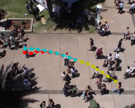
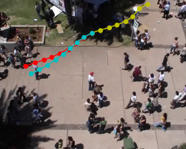
In all three examples, we can see that the predicted trajectories (cyan) are very close to the ground-truth trajectories (red), indicating good performance. We can also see that the dataset includes many examples where the pedestrian stands still or stays in the same area, as in the second image.

Multimodal Trajectory Prediction Conditioned on Lane-Graph Traversals

Paper: https://doi.org/10.48550/arXiv.2106.15004 [3]

Repository: https://github.com/nachiket92/PGP [4]

Overview

This paper introduces Prediction via Graph-Based Policy (PGP), an improvement on multimodal regression for trajectory prediction [3].

While standard multimodal regression aggregates the entirety of the graph representation of the map, the new method instead takes a subset of graph data that is more relevant to the vehicle and selectively aggregates this data [3].

In addition to lateral motion (acceleration, braking, etc.), the model also examines variations in longitudinal motion such as lane changes, utilizing a latent variable [3].

The model utilizes a graph encoder to encode node and agent features, a policy header to determine probable routes, and a trajectory decoder to determine a likely trajectory from this data [3].

Technical Details

The model consists of a graph encoder, policy header, and trajectory decoder [3].

The graph encoder utilizes three GRU encoders to encode the nodes, agents, and motion [3]. An example of such an encoder (lines 43-45 of pgp_encoder.py in the source) is as follows: [4]

# Node encoders
self.node_emb = nn.Linear(args['node_feat_size'], args['node_emb_size'])
self.node_encoder = nn.GRU(args['node_emb_size'], args['node_enc_size'], batch_first=True)

Since agents respond to other nearby agents in traffic, node encodings are updated using information from agent encodings within a certain distance, utilizing multi-head attention to do so [3]; the layers are implemented in lines 51-56 of pgp_encoder.py in the source as: [4]

# Agent-node attention
self.query_emb = nn.Linear(args['node_enc_size'], args['node_enc_size'])
self.key_emb = nn.Linear(args['nbr_enc_size'], args['node_enc_size'])
self.val_emb = nn.Linear(args['nbr_enc_size'], args['node_enc_size'])
self.a_n_att = nn.MultiheadAttention(args['node_enc_size'], num_heads=1)
self.mix = nn.Linear(args['node_enc_size']*2, args['node_enc_size'])

The attention output is concatenated with the original encoding and a GNN is then used to aggregate node context [3]. The GNN is implemented using graph attention (GAT) in lines 222-251 of pgp_encoder.py in the source as: [4]

class GAT(nn.Module):
    """
    GAT layer for aggregating local context at each lane node. Uses scaled dot product attention using pytorch's
    multihead attention module.
    """
    def __init__(self, in_channels, out_channels):
        """
        Initialize GAT layer.
        :param in_channels: size of node encodings
        :param out_channels: size of aggregated node encodings
        """
        super().__init__()
        self.query_emb = nn.Linear(in_channels, out_channels)
        self.key_emb = nn.Linear(in_channels, out_channels)
        self.val_emb = nn.Linear(in_channels, out_channels)
        self.att = nn.MultiheadAttention(out_channels, 1)

    def forward(self, node_encodings, adj_mat):
        """
        Forward pass for GAT layer
        :param node_encodings: Tensor of node encodings, shape [batch_size, max_nodes, node_enc_size]
        :param adj_mat: Bool tensor, adjacency matrix for edges, shape [batch_size, max_nodes, max_nodes]
        :return:
        """
        queries = self.query_emb(node_encodings.permute(1, 0, 2))
        keys = self.key_emb(node_encodings.permute(1, 0, 2))
        vals = self.val_emb(node_encodings.permute(1, 0, 2))
        att_op, _ = self.att(queries, keys, vals, attn_mask=~adj_mat)

        return att_op.permute(1, 0, 2)

With the node encoding completed, the data will then pass through the policy header, which utilizes an MLP to output probabilities for each node’s edges [3]; the layers are implemented in lines 37-45 of pgp.py in the source as: [4]

# Policy header
self.pi_h1 = nn.Linear(2 * args['node_enc_size'] + args['target_agent_enc_size'] + 2, args['pi_h1_size'])
self.pi_h2 = nn.Linear(args['pi_h1_size'], args['pi_h2_size'])
self.pi_op = nn.Linear(args['pi_h2_size'], 1)
self.pi_h1_goal = nn.Linear(args['node_enc_size'] + args['target_agent_enc_size'], args['pi_h1_size'])
self.pi_h2_goal = nn.Linear(args['pi_h1_size'], args['pi_h2_size'])
self.pi_op_goal = nn.Linear(args['pi_h2_size'], 1)
self.leaky_relu = nn.LeakyReLU()
self.log_softmax = nn.LogSoftmax(dim=2)

Loss for the policy header is calculated using negative log likelihood [3], implemented in pi_bc.py in the source [4].

Once possible future routes are determined, multi-head attention is utilized again for selective aggregation of context to form possible trajectories and the motion that will be undertaken (which may vary for a given trajectory) [3]. The aggregator layers are implemented in lines 51-56 of pgp.py in the source as: [4]

# Attention based aggregator
self.pos_enc = PositionalEncoding1D(args['node_enc_size'])
self.query_emb = nn.Linear(args['target_agent_enc_size'], args['emb_size'])
self.key_emb = nn.Linear(args['node_enc_size'], args['emb_size'])
self.val_emb = nn.Linear(args['node_enc_size'], args['emb_size'])
self.mha = nn.MultiheadAttention(args['emb_size'], args['num_heads'])

Finally, the decoder utilizes an MLP and K-means clustering to output predicted trajectories [3], with the implementation of the MLP layers in lines 33-35 of lvm.py in the source as: [4]

self.hidden = nn.Linear(args['encoding_size'] + args['lv_dim'], args['hidden_size'])
self.op_traj = nn.Linear(args['hidden_size'], args['op_len'] * 2)
self.leaky_relu = nn.LeakyReLU()

Loss for the decoder is calculated using average displacement error [3], implemented in min_ade.py in the source [4]. The total loss is the sum of the losses of the policy header and the decoder [3].

The metrics the model are evaulated on are the minimum average displacement error (minADE) of each point in the predicted trajectory from the ground-truth trajectory [3], and the miss rate, which tracks deviations of more than 2 m from said ground-truth trajectory [3]. Both metrics are evaluated with the top 5 and top 10 predicted trajectories, resuting in four metrics in total; in all cases, a lower value is desired [3].

Setup

Navigate to the ProjectRoot/Models directory and run the command

git clone https://github.com/nachiket92/PGP.git

to clone the repository [4]. Most of the following commands are from the repository’s README.md [4], but tailored to work with the project.

Follow the instructions in the repository’s README.md [4] to set up the virtual environment. However, when installing Pytorch, run

conda install pytorch==1.7.1 torchvision==0.8.2 torchaudio==0.7.2 cudatoolkit=10.1 -c pytorch -c nvidia

instead of the command provided by the README.md [4] to enable proper CUDA support; the model appears to assume CUDA is available and will not work properly otherwise.

Navigate to the ProjectRoot/Data and run the commands

mkdir nuScenes
mkdir nuScenesPreprocessed

Follow the instructions in the repository’s README.md [4] to download and set up the nuScenes dataset. Afterwards, run the command

python preprocess.py -c configs/preprocess_nuscenes.yml -r ../../Data/nuScenes -d ../../Data/nuScenesPreprocessed/

to preprocess the data. Note that this will take several hours to run and will require a large amount of storage; the Google Cloud Project VM that was used has 500 GB of disk space allocated, which is sufficient. Should there be insufficient GPU memory, open ProjectRoot/Models/PGP/configs/preprocess_nuscenes.yml and reduce the value of num_workers. The default value was 4, which we had to reduce to 2 to have sufficient memory.

Download the pre-trained weights, which are available via a link on the repository’s README.md [4], and save it to the ProjectRoot/Checkpoints directory. Note that while the weights are a .tar file, the file does not actually appear to be a tarball and thus cannot be extracted; rather, the entire file is to be passed into the model.

For the studies which were run on the model, navigate to ProjectRoot/Outputs and run the command

mkdir PGP

Navigate to this newly-created directory and run the commands

mkdir Pre-Trained
mkdir Original
mkdir Encoder_GAT_4
mkdir Finetune

Studies

All training and evaluation commands are run in the ProjectRoot/Models/PGP directory.

Studies were conducted on the nuScenes dataset [7], which the model is designed to work with. The first goal was to utilize the pre-trained weights [4] to evaluate the model and visualize output predictions to see if results from the paper could be replicated. The next goal was to train the model from scratch to ensure that results match those of the pre-trained weights. The model was trained from scratch with the command

python train.py -c configs/pgp_gatx2_lvm_traversalOriginal.yml -r ../../Data/nuScenes -d ../../Data/nuScenesPreprocessed/ -o ../../Outputs/PGP/Original/ -n 100

and the pre-trained and trained-from-scratch models were evaluated with the commands

python evaluate.py -c configs/pgp_gatx2_lvm_traversalOriginal.yml -r ../../Data/nuScenes -d ../../Data/nuScenesPreprocessed/ -o ../../Outputs/PGP/Pre-Trained/ -w ../../Checkpoints/PGP_lr-scheduler.tar

python evaluate.py -c configs/pgp_gatx2_lvm_traversalOriginal.yml -r ../../Data/nuScenes -d ../../Data/nuScenesPreprocessed/ -o ../../Outputs/PGP/Original/ -w ../../Outputs/PGP/Original/checkpoints/best.tar

The model was originally trained using the configuration file pgp_gatx2_lvm_traversal.yml [4], but due to the setup for the next study, the configuration file needed to replicate this training is instead pgp_gatx2_lvm_traversalOriginal.yml, though the hyperparameters are unchanged.

Afterwards, the first study that was conducted was regarding the number of GAT layers. The model utilizes two of such layers [4], with the article noting that increasing the number of layers has little effect and even “ambiguous results” [3]; the article shows results with one GAT layer and with two, indicating that the additional layer slightly increases minimum ADEs but slightly decreases miss rates. With this in mind, we wanted to see what would happen if the number of GAT layers was increased further. To this effect, the configuration file pgp_gatx2_lvm_traversal.yml (located in ProjectRoot/Models/PGP/configs) was copied and the original file renamed to pgp_gatx2_lvm_traversalOriginal.yml; the number of GAT layers, expressed in pgp_gatx2_lvm_traversal.yml as num_gat_layers under the encoder parameters [4], was doubled from 2 to 4. The modified model was trained with the command

python train.py -c configs/pgp_gatx2_lvm_traversal.yml -r ../../Data/nuScenes -d ../../Data/nuScenesPreprocessed/ -o ../../Outputs/PGP/Encoder_GAT_4 -n 100

and evaluated with the command

python evaluate.py -c configs/pgp_gatx2_lvm_traversal.yml -r ../../Data/nuScenes -d ../../Data/nuScenesPreprocessed/ -o ../../Outputs/PGP/Encoder_GAT_4/ -w ../../Outputs/PGP/Encoder_GAT_4/checkpoints/best.tar

Additionally, after the model was trained from scratch using the original hyperparameters (i.e. two GAT layers [3]), the model created the directory checkpoints in ProjectRoot/Outputs/PGP/Original and saved the training weights for each epoch, in addition to tracking the checkpoint with the best results. Based off of the timestamps as to when the optimal checkpoint best.tar was last updated, the best checkpoint was determined to be designated as 42.tar, so we were then interested in seeing if it was possible to finetune the model and improve performance further. Hence, the configuration file pgp_gatx2_lvm_traversalOriginal.yml in ProjectRoot/Models/PGP/configs was copied, with the new version renamed to pgp_gatx2_lvm_traversalFinetune.yml; the learning rate was then decreased by a factor of 40 from the default .001 to 0.000025 and the finetuning commenced from the epoch immediately before the best checkpoint, 41.tar. The finetuning was conducted with the command

python train.py -c configs/pgp_gatx2_lvm_traversalFinetune.yml -r ../../Data/nuScenes -d ../../Data/nuScenesPreprocessed/ -o ../../Outputs/PGP/Finetune/ -n 100 -w ../../Outputs/PGP/Original/checkpoints/41.tar

and evaluated with the command

python evaluate.py -c configs/pgp_gatx2_lvm_traversalFinetune.yml -r ../../Data/nuScenes -d ../../Data/nuScenesPreprocessed/ -o ../../Outputs/PGP/Finetune/ -w ../../Outputs/PGP/Finetune/checkpoints/best.tar

Results

The paper noted that the model has minimum ADEs of 1.30 and 1.00 for top 5 and top 10 predicted trajectories, as well as miss rates of .61 and .37 for top 5 and top 10 predicted trajectories [3], and we wanted to see if these results were replicable.

For increased precision of output values, the file evaluator.py located in ProjectRoot/Models/PGP/train_eval [4] was modified on line 81, replacing .02f with .05f, thereby increasing precision from two decimal places to five.

Evaluation outputs are stored as text files in the respective output directories as ProjectRoot/Outputs/PGP/[TYPE]/results/results.txt.

The outputs for the pre-trained model are:

min_ade_5: 1.27230
min_ade_10: 0.94289
miss_rate_5: 0.52892
miss_rate_10: 0.34288
pi_bc: 3.14598

This appears to replicate the results of the paper, achieving outputs with slightly better performance.

The outputs for the trained-from-scratch model are:

min_ade_5: 1.27727
min_ade_10: 0.94902
miss_rate_5: 0.52826
miss_rate_10: 0.34012
pi_bc: 1.83836

ADEs seem to be slightly higher than the pre-trained model, while miss rates seem to be slightly lower. However, the values are still close to those of the pre-trained weights and are still better than those of the paper.

The outputs for the model with four GAT layers are:

min_ade_5: 1.28691
min_ade_10: 0.95485
miss_rate_5: 0.51388
miss_rate_10: 0.33791
pi_bc: 1.93244

ADEs seem to be higher than both the pre-trained and trained-from-scratch models, while miss rates seem to be slightly lower than both. Results are still better than those of the paper, and the trends shown here (more layers resulting in higher ADEs and lower miss rates) follow the trends shown in the paper, which compared one GAT layer versus two.

The outputs for the finetuned model are:

min_ade_5: 1.27362
min_ade_10: 0.94978
miss_rate_5: 0.51587
miss_rate_10: 0.33437
pi_bc: 1.85104

Although the ADE performance of the finetuned model does not quite reach that of the pre-trained model, it does outperform the trained-from-scratch and four-GAT-layer models in terms of the top 5 predictions. However, its performance appears to be the worst of the four models when it comes to the ADE with top 10 predictions. That said, when it comes to miss rate, the finetuned model appears to perform better with top 10 predictions, outperforming all other models; for miss rate with top 5 predictions, the finetuned model does not perform as well as the model with four GAT layers, but outperforms the others.

Additionally, the model allowed for the outputs to be visualized as .gifs, which were generated with the commands

python visualize.py -c configs/pgp_gatx2_lvm_traversalOriginal.yml -r ../../Data/nuScenes -d ../../Data/nuScenesPreprocessed/ -o ../../Outputs/PGP/Pre-Trained/ -w ../../Checkpoints/PGP_lr-scheduler.tar

python visualize.py -c configs/pgp_gatx2_lvm_traversalOriginal.yml -r ../../Data/nuScenes -d ../../Data/nuScenesPreprocessed/ -o ../../Outputs/PGP/Original/ -w ../../Outputs/PGP/Original/checkpoints/best.tar

python visualize.py -c configs/pgp_gatx2_lvm_traversal.yml -r ../../Data/nuScenes -d ../../Data/nuScenesPreprocessed/ -o ../../Outputs/PGP/Encoder_GAT_4/ -w ../../Outputs/PGP/Encoder_GAT_4/checkpoints/best.tar

python visualize.py -c configs/pgp_gatx2_lvm_traversalFinetune.yml -r ../../Data/nuScenes -d ../../Data/nuScenesPreprocessed/ -o ../../Outputs/PGP/Finetune/ -w ../../Outputs/PGP/Finetune/checkpoints/best.tar

In all visualizations, the left view shows the movement of the vehicle itself, the middle view shows the predicted trajectories, and the right view shows the ground-truth. These visualizations are stored in the respective output directories as ProjectRoot/Outputs/PGP/[TYPE]/results/gifs/[GIF]; there appear to be 13 .gifs in each directory, numbered example0.gif to example12.gif. Shown here are the example3.gif visualizations of the models, though it is worth noting that the files were manually renamed.

Pre-trained:

Trained from scratch:

Four GAT layers:

Finetuned:

Overall, the pre-trained model performs the best when it comes to ADE, while the model with four GAT layers and the finetuned model perform the best when it comes to miss rate.

Trajectron++: Dynamically-Feasible Trajectory Forecasting With Heterogeneous Data

Paper: https://doi.org/10.48550/arXiv.2001.03093 [5]

Repository: https://github.com/StanfordASL/Trajectron-plus-plus [6]

Overview

This paper introduces a graph-structure recurrent model called Trajectron++. which predicts the trajectories of any number of agents. Trajectron++ incorporates agent dynamics and heterogeneous data (e.g. semantic maps) [5].

Unlike previous models, Trajectron++ accounts for dynamics constraints on agents and incorporates different kinds of environmental information (e.g. maps) [5].

Results

SGNet Colab Demonstration

Project Results

Project Video

References

[1] Wang, Chuhua, et al. “Stepwise Goal-Driven Networks for Trajectory Prediction”. ArXiv, IEEE, 27 Mar 2022, https://doi.org/10.48550/arXiv.2103.14107. Papers with Code, Papers with Code, 25 Mar 2021, www.paperswithcode.com/paper/stepwise-goal-driven-networks-for-trajectory, accessed 29 Jan 2023.

[2] Wang, Chuhua and Mingze Xu. “SGNet.pytorch.” GitHub, GitHub, www.github.com/ChuhuaW/SGNet.pytorch. Papers with Code, Papers with Code, 25 Mar 2021, www.paperswithcode.com/paper/stepwise-goal-driven-networks-for-trajectory, accessed 29 Jan 2023.

[3] Deo, Nachiket, et al. “Multimodal Trajectory Prediction Conditioned on Lane-Graph Traversals.” ArXiv, ArXiv, 15 Sep 2021, www.doi.org/10.48550/arXiv.2106.15004. Papers with Code, Papers with Code, 28 Jun 2021, www.paperswithcode.com/paper/multimodal-trajectory-prediction-conditioned, accessed 26 Feb 2023.

[4] Deo, Nachiket. “PGP.” GitHub, GitHub, www.github.com/nachiket92/PGP. Papers with Code, Papers with Code, 28 Jun 2021, www.paperswithcode.com/paper/multimodal-trajectory-prediction-conditioned, accessed 26 Feb 2023.

[5] Salzmann, Tim, et al. “Trajectron++: Dynamically-Feasible Trajectory Forecasting With Heterogeneous Data” ArXiv, ECCV, 13 Jan 2021, www.doi.org/10.48550/arXiv.2001.03093. Papers with Code, Papers with Code, 2020, www.paperswithcode.com/paper/trajectron-multi-agent-generative-trajectory, accessed 25 Mar 2023.

[6] Ivanovic, Boris and Mohamed Zahran. “Trajectron-plus-plus.” GitHub, GitHub, www.github.com/StanfordASL/Trajectron-plus-plus. Papers with Code, Papers with Code, 2020, www.paperswithcode.com/paper/trajectron-multi-agent-generative-trajectory, accessed 25 Mar 2023.

[7] nuScenes. Motional, 2020, www.nuscenes.org. Accessed 26 Feb 2023.