NeRF Models

This project delves into the cutting-edge technology behind Image-generative AIs, particularly Neural Radiance Fields (NeRF). We will investigate the research and methodologies behind NeRF and its applications in 3D scene reconstruction and rendering. Additionally, we will provide a hands-on, toy implementation using Pytorch and Google Colab.

• What is NeRF?
• Dataset
• A Closer Look into NeRF
  • NeRF Overview
  • NeRF Model
  • Rendering of the Radiance Field
  • Optimizations in the Neural Radiance Field
  • Architecture
• Innovations
  • Mip-NeRF
  • Instant NeRF
• Generate NeRF
  • Video Demo
• Discussion
• References

What is NeRF?

NeRF is a technique for synthesizing novel views of a scene from a set of input images using deep learning. It was introduced in NeRF: Representing Scenes as Neural Radiance Fields for View Synthesis by Ben Mildenhall, Pratul P. Srinivasan, Matthew Tancik, Jonathan T. Barron, Ravi Ramamoorthi, and Ren Ng in 2020.

The main idea of NeRF is to represent a scene as a continuous volumetric function, which maps 3D coordinates to a density and a color value. This function can be parameterized by a neural network that learns to generate different views of the scene. NeRF optimizes the network to minimize the difference between the rendered images and the input images in both color and density

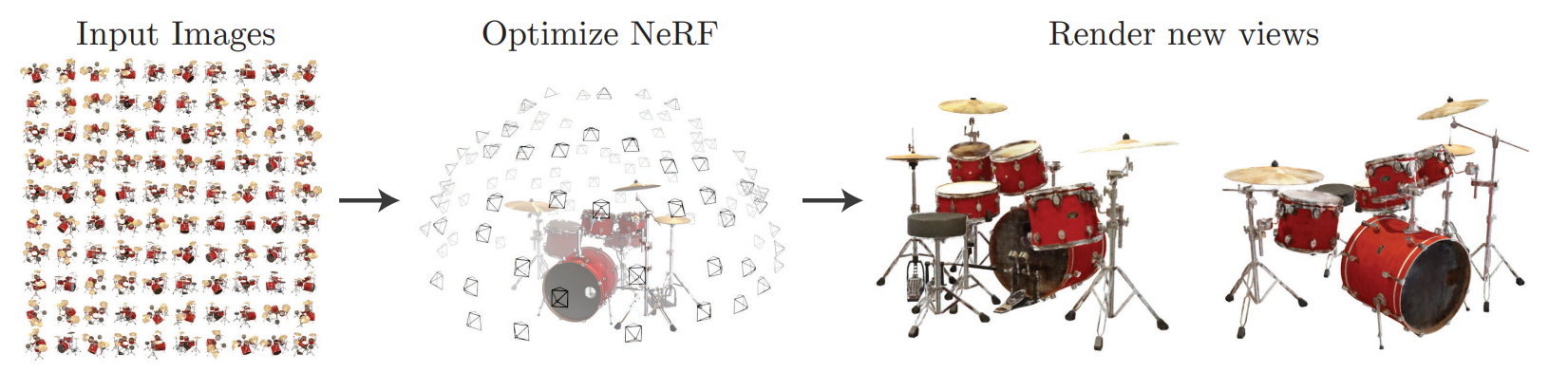
Fig 1. The General Idea of NeRF.

The main advantage of NeRF is that it can generate high-quality novel views of a scene with a relatively small number of input images. It has shown great potential in various applications, including 3D reconstruction, virtual reality, and computer graphics. However, there are also limitations of NeRF that it’s computationally intensive, and improvements are still being made to address its limitations, such as Instant NeRF, pixelNeRF, and Mip-NeRF.

Even though NeRF models have recently added many advanced optimizations and features, we will focus on a relatively simple implementation with a focuses on the core advancements.

Dataset

In order to explore different NeRF models with varying implementations. This project will use primarily the Lego NeRF and the Fern Nerf. There are also additions of photos taken by our team to show the power of NeRF models.

A Closer Look into NeRF

NeRF Overview

The main idea of NeRF involves taking the 5D input $(x, y, z, \theta, \phi)$ in which $(x, y, z)$ are 3D coordinates of the camera and $(\theta, \phi)$ are viewing direction angles of the given camera. In more detail, $x$ usually refers to the horizontal axis, $y$ usually to the vertical axis, and $z$ usually to the depth axis. These 3D coordinates are taken as input to evaluate the radiance and density at each point in the scene. $\theta$ is taken as a polar angle in spherical coordinates that represents the inclination of the viewing direction vector with respect to the positive z-axis. It has a range of 0 to 180 degrees (or 0 to $\pi$ radians). $\phi$ is taken as the azimuthal angel in spherical coordinates that represents the orientation of the viewing direction vector with respect to the positive x axis.. It has a range of 0 to 360 degrees (or 0 to w $\pi$ radians). Both $\theta$ and $\phi$ help to describe the viewing direction of the given camera.

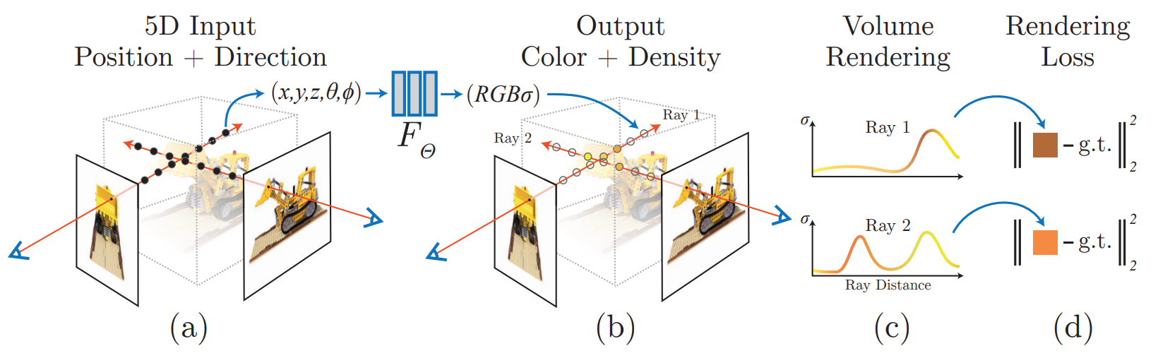
Fig 2. NeRF models in a closer view.

After collecting the 5D input $(x, y, z, \theta, \phi)$, a neural network is utilzied to model the radiation field, more specifically, RGB$\sigma$. In this way, the size of the space we represent will not affect the space capacity needed to represent the radiation field. The radiation field is also continuous as follows:

NeRF Model

The neural network can be represented as follows:

class NerfModel(nn.Module):
    def __init__(self, embedding_dim_pos=10, embedding_dim_direction=4, hidden_dim=128):
        super(NerfModel, self).__init__()
        # Define blocks of layers
        self.block1 = self.create_block(embedding_dim_pos * 6 + 3, hidden_dim, layers=4)
        self.block2 = self.create_block(embedding_dim_pos * 6 + hidden_dim + 3, hidden_dim, layers=3, output_dim=hidden_dim + 1)
        self.block3 = self.create_block(embedding_dim_direction * 6 + hidden_dim + 3, hidden_dim // 2, layers=1)
        self.block4 = self.create_block(hidden_dim // 2, 3, layers=1, activation=nn.Sigmoid())

        self.embedding_dim_pos = embedding_dim_pos
        self.embedding_dim_direction = embedding_dim_direction

    def create_block(self, input_dim, hidden_dim, layers=1, output_dim=None, activation=nn.ReLU()):
        block = []
        for _ in range(layers):
            block.extend([nn.Linear(input_dim, hidden_dim), activation])
            input_dim = hidden_dim
        if output_dim is not None:
            block.append(nn.Linear(hidden_dim, output_dim))
            if activation != nn.ReLU():
                block.append(activation)
        return nn.Sequential(*block)
        @staticmethod

    # Define the positional encoding function    
    def pos_enc(input_tensor, enc_dim):
        output = [input_tensor]
        for idx in range(enc_dim):
            output.append(torch.sin(2 ** idx * input_tensor))
            output.append(torch.cos(2 ** idx * input_tensor))
        return torch.cat(output, dim=1)

    # Define the forward pass
    def forward(self, obj, direction):
        # Apply positional encoding to the input object and direction
        obj_enc = self.pos_enc(obj, self.pos_embed_dim)
        dir_enc = self.pos_enc(direction, self.dir_embed_dim)
        hidden = self.block1(obj_enc)
        combined = self.block2(torch.cat((hidden, obj_enc), dim=1))
        hidden, sigma = combined[:, :-1], self.relu(combined[:, -1])
        hidden = self.block3(torch.cat((hidden, dir_enc), dim=1))
        color = self.block4(hidden)
        return color, sigma    

Rendering of the Radiance Field

In order to get the expected color $C(\mathbf{r})$ of camera ray $\mathbf{r}(t) = \mathbf{o} + t\mathbf{d}$ with near and far bounds $t_n$ and $t_f$, the following fuction is used:

$t$ is represented as the depth of the radiation field and $T(t)$ is represented as the intensity of light. It can be found that $T(t)$ decreases with the distance $t$ increases.

However, since it’s very computationally expensive to have a continuous function representation in PyTorch, a discrete method is used to estimate the result of color instead:

in which $\delta_i = t_{i+1} - t$ is the distance between adjacent samples. In this way, the rays are divided into N small intervals. We then randomly sample a point in each interval and perform a weighted summation of colors to get the final color.

Optimizations in the Neural Radiance Field

Positional Encoding

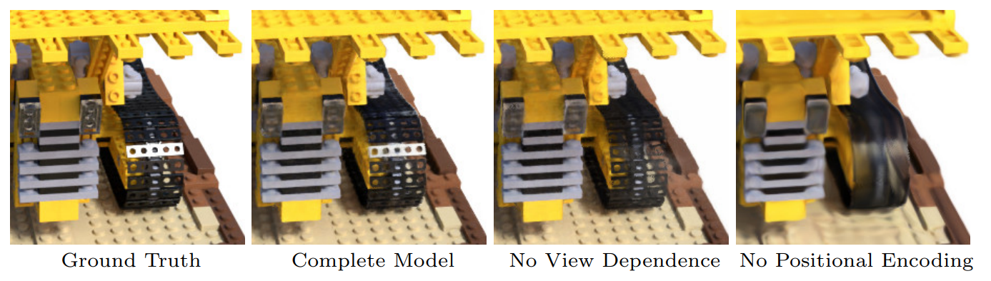
Fig 4. Positional Encoding.

The positional encoding is very similar to the mapping in Transformer in which the coordinates and viewing angles are expressed in a higher dimension as network input to solve the problem of blurred rendered images. The encoding function is the following:

In the above function of positional encoding, the function is applied separately to the 3D coordinates (x) and the 3 components of the Cartesian viewing direction unit vector (d). The coordinates are normalized to lie in the range [-1, 1], and the viewing direction components also lie within this range by construction. This is significant in formulating the function

since $F’_0\theta$ is a Multi-Layer Perceptron(MLP) and $\gamma$ is a mapping from $\R$ to higher dimension space $\R^{2L}$. Formulating $F\theta$ as two finctions improves the performance in representing neural scenes.

Hierachical Volume Sampling

Furthermore, because the density distribution in the space is uneven, if the rays are uniformly and randomly sampled, the rendering efficiency will be relatively low. In this case. the rays may pass through fewer high-density points after passing through a long distance. From the above analysis, we can see that the entire rendering process is nothing more than a weighted summation of the colors of the sampling points on the ray. In this case, the weight $w_i = T_i(1 - exp(-\sigma_i\delta_i))$.

We can weight the colors in the rendering formula with $w_i$ as the probability of sampling in the corresponding interval. We can then train a fine and a coarse network to improve the efficienty. The coarse network use $w_i$ as estimations to the sampling probability. The fuction is as follow:

In the fine network, we utilized

function which uses $\hat{w}_i$ as the sampling probability for $N_f$ points. This way, a better result can be produced.

Architecture

The architecture of NeRF is to have the coordinates $\mathbf{x} = (x, y, z)$ into a 60-dimensional vector as an input to the fully connected network to get the density $\sigma$. The viewing angle $\mathbf{d} = (\theta, \phi)$ is then added to the output of the network. After getting through the MLP, RGB value can be obtained. Below is an image of the architecture.

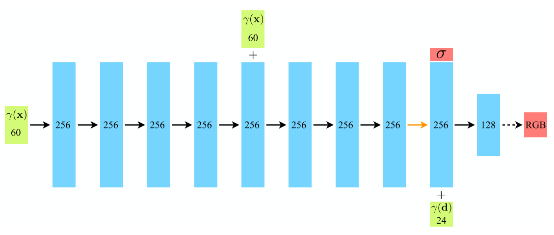
Fig 3. NeRF Architecture.

Innovations

Mip-NeRF

Mip NeRF(Multiscale Inference and Prediction Neural Radiance Fields) has innnovations over the original NeRF to improve the performance.

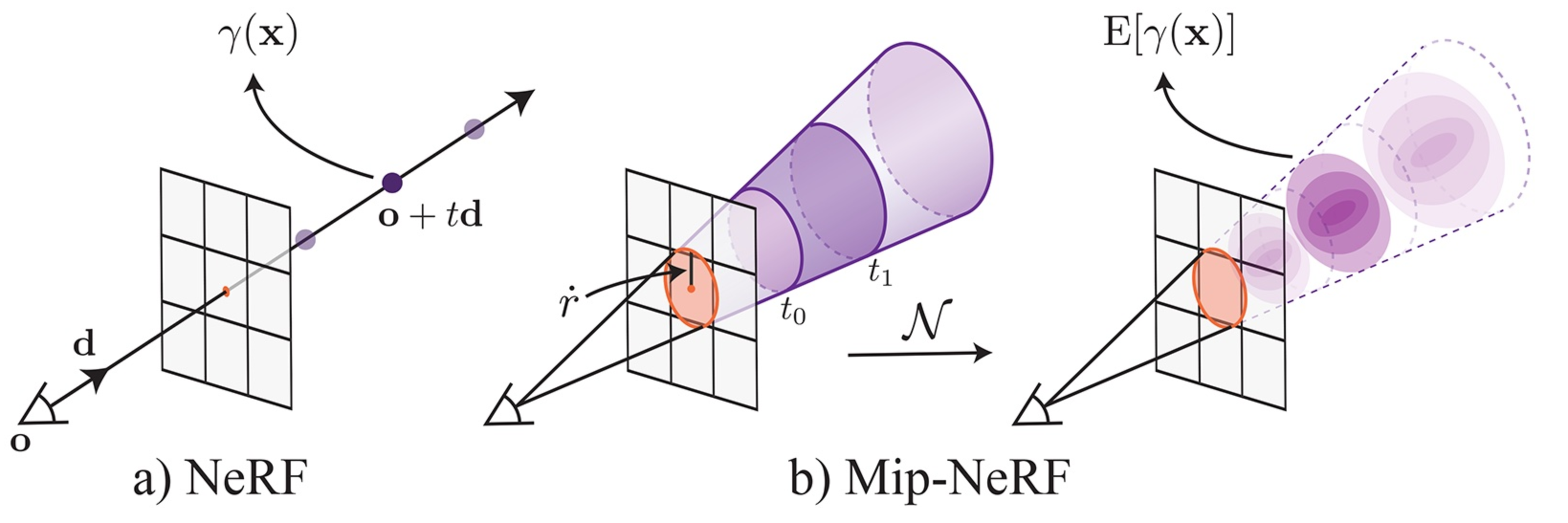
Fig 5. NeRF vs Mip-NeRF.

One of the main contributions of Mip-NeRF is cone tracing, the original rendering procedure of NeRF is to have a ray per pixel, however, in Mip-NeRF, the procedure is to have a 3D conical frustum per pixel. The conical frustums are then characterized using an integrated positional encoding (IPE). This process involves approximating the frustum with a multivariate Gaussian and subsequently calculating the integral $E[γ(x)]$ over the positional encodings of the coordinates within the Gaussian in a closed-form manner.

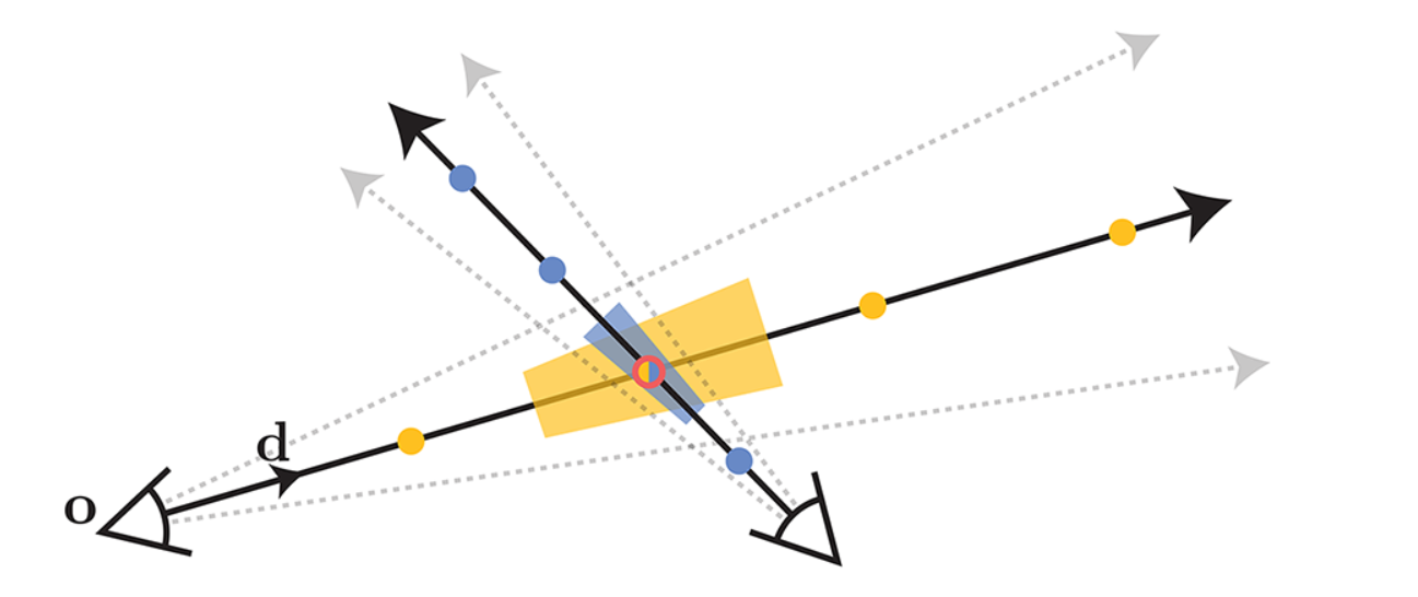
Fig 6. Mip-NeRF Utilized Cone Instead of a Ray for Each Pixel.

The Featurization procedure is also different, the original NeRF involves obtaining point-sampled positional encoding features (depicted as dots) along each pixel’s ray. However, because these point-sampled features don’t have shape and size of the volume viewed by each ray, ambiguity can occur when different cameras capture the same position at varying scales. In this case, NeRF’s performance will be negatively impacted. Instead, Mip-NeRF utilizes cones instead of rays and explicitly models the volume of each sampled conical frustum (represented as trapezoids), effectively addressing this ambiguity.

There are also differences in hierarchical sampling procedure, NeRF utilizes two distict MLPs that one is “coarse” and one is “fine”. There are also uneven samples of “coarse” and “fine” in the original NeRF. In Mip-NeRF, there’s only a single MLP with equal samples for “coarse” and “fine”. The even samples are a result of the single MLP which is shown in the following optimization problem:

In this way, the model size can be cut in half, renderings becomes more accurate, sampling is more efficient, and the overal structure becomes simplier.

Instant NeRF

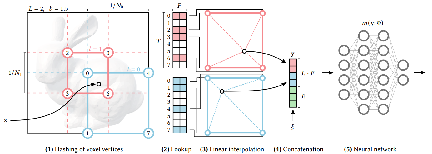
Fig 8. Instant NeRF.

Instant NeRF utilizes a multi-layer hash encoding to solve the difficulties of storing latent features. In simplier way, it’s uses a multi resolution hash table to store features.

Given an input coordinate $x$, the first step in the multiresolution hash encoding process is to locate the surrounding voxels at $L$ different resolution levels. Once having identified these voxels, we assign indices to their corners by hashing their integer coordinates.

Then we look up the corresponding $F$-dimensional feature vectors from the hash tables $\theta l$ for each index. This makes it possible to store the features in the Hash Table.

The Linear Interpolation step linearly interpolate the $F$-dimensional feature vectors based on the relative position of the input coordinate $x$ within its respective $l$-th voxel.

After the linear interpolation, we then concatenate the resulting feature vectors from each resolution level. We will also include auxiliary inputs $\xi \in \R^E$ to create the encoded MLP (Multilayer Perceptron) input $y \in \R^{LF + E}$.

The final step is to evaluate the encoded MLP input using a multilayer perceptron.

Overall, with these innovations, Instant NeRF makes it possible to render high-resolusion 3D scene in just a few seconds. There are many potential applications of Instant NeRF, including reconstruct scenes for 3D maps and video conferences.

Generate NeRF

Fig 8. NeRF of a toy car.

Fig 8. NeRF of a poster, made by nerfstudio. Once the model is fully trained, it is relatively simple for the NeRF model to generate 3D scenes. Similarly to Assignment 4, we can generate the 3D views of a toy car. We can also generate the 3D views of the poster.

Video Demo

Discussion

Even thoug Neural Radiance Fields (NeRF) is a powerful method for synthesizing novel views of a scene from a set of input images, there are also some limitations of NeRF. NeRF is computational expensive that it requires large VRAM and time to successfully train a model. It also has limited generalization that NeRF models are scene-specific such that a new model must be trained for a new scene.

References

Papers:

• NeRF: Representing Scenes as Neural Radiance Fields for View Synthesis
  • Github
• Instant Neural Graphics Primitives with a Multiresolution Hash Encoding
  • Github
• Mip-NeRF: A Multiscale Representation for Anti-Aliasing Neural Radiance Fields
  • Github