Mushroom Classification Project Proposal
Mushrooms can be delicious, symbols in popular culture, and found nearly anywhere, but dealing with them safely can be tricky because while many look the same to the untrained eye, some mushrooms are extremely poisonous. Here, we attempted to classify 1394 types of mushrooms with as little as 3 images for some species using various deep learning methods.
Introduction
Code: https://colab.research.google.com/drive/1Mi0htyUSBqYYqXBgzx5SXVqvke1CHy2z?usp=sharing Vide0: https://youtu.be/Xq15gpnjjNw
Mushrooms are a specific form of fungus that have had their image rise in popular culture as a hip symbol for peace, health, and for their occasional hallucinogenic properties. This has caused a rise in mushroom foraging, a practice of going out into swampy or recently rained on areas to gather mushrooms, as well as commercial mushroom farming where fungal environments are created to grow certain mushrooms for eating. In both of these cases, it is common for multiple types of mushrooms to appear given how easily dispersable fungal spores can be. This can be dangerous as certain mushrooms can appear similar to the untrained eye but can be very poisonous if misclassified. Our goal as mushroom fans ourselves is to develop a model that can help classify mushrooms so that we can continue foraging safely, without having to learn textbooks worth of knowledge to avoid being poisoned.
The Dataset
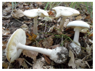
Fig 1. Poisonous-Mushroom: Species Amanita Phalloides [0].
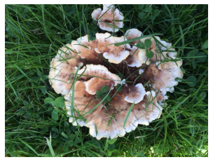
Fig 2. Flat-Mushroom: Species Abortiporus Biennis [0].
Data Engineering
Mushrooms are generally not found completely isolated on a slate rock, posed for the perfect picture with an even background. They are amidst damp soil, rotting leaves, and all kinds of other foliage. Because of this, we will need to work with our data such that our model can detect where the mushroom is by focusing solely on the shape of the mushroom. Then, we can continue with the mushroom’s many various colors and orientations to simply generate more data and not overfit to certain viewpoints. Our biggest challenge is the diversity of ourdataset: we have 89760 images split unevenly amongst 1394 categories. In order to overcome our dataset diversity and small sample size per category, we will attempt to increase our dataset with two augmentation transforms that will aim to make the model focus on shape and simply generate more data through various positional changes. Additionally, because our dataset has so few images for some labels, these augmentations will also help regularize some of the learning to not overfit our limited dataset.
Aiming for Shape
This transorm contains the grayscale and Random Solarize transformations in an attempt to make the model focus on the shapes of the mushrooms in the image.
Grayscale
Grayscaling an image in a basic sense does exactly what it sounds like and makes a colored image have only shades of gray, removing all color. In reality, it collapses the initial three RGB channels into a single channel to remove any indication of color. For the purposes of our dataset we still want a three channel input for the dimensionality of our different models so te image will still hav threee channels but they will be the same where R=G=B.
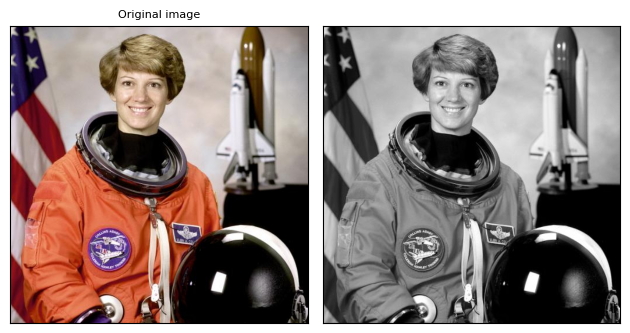
Fig 3. Grayscaled example [4].
Random Solarize
On top of grayscaling we will use a tranform called Random Solarization that will invert pixel values above a certain threshold with probability p. The idea behind this transformation is that we don’t want the model to learn features solely on edge case pixel values that could highlight bright lights or colors over features of the mushrooms themselves. Therefore, with probability p (set to .9 in our model) we will invert the top most pixel values above the threshold 192 (out of 256 for RGB). We chose the hyperparameters .9 and 192 because we want this transformation to happen often since are concatonating these images with the original data and because 192 is the 75th percentile of pixel values (in general, not calculated over image appearance probability). After these two transformations we will append this grayscaled, solarized dataset onto our original, doubling out dataset size.
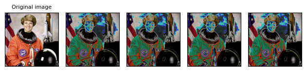
Fig 4. Random Solarize Example [4].
Increasing Dataset through Positional Augmentation
This transorm contains the random rotation, horizonatal flip, and color jitter transformations in an attempt to augment our data enough to squeeze more information out of our limited dataset.
Random Rotation
the Random Rotation augmentation rotates an image randomly between a min and max degree range. We set the range to be 0 to 180. This is an important augmentation particularly because some of the mushroom images in this dataset are always in a certain orientation, i.e. growing straight up vertically versus 45 degrees out from a tree trunk. This is not necessarily because the mushrooms always grow this way, in which case it would be a feature, but are just only photographed from that perepective and therefore we don’t want to overfit on just the angle of the stem. Additionally, some of the mushrooms are very flat and turning them a random amount just gives us a new data point from a different orientation the image could’ve been taken from.
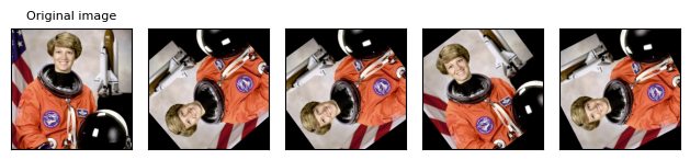
Fig 5. Random Rotation Example [4].
Horizontal Flip
The orizontal Flip augmentation flips the image horizontally with probability p. This augmentation has a very similar purpose to Random Rotation in that it will give us a new perspective and prevent overfitting on certain mushroom orientations common in the dataset.
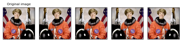
Fig 6. Random Horizontal Flip Example [4].
Color Jitter
The Color Jitter augmentation is the last of this series of transforms. Color Jitter randomly changes the brightness, contrast, saturation, and hue of an image. The amount to jitter each factor is chosen uniformly from [max(0,1-factor), 1 + factor]. We chose a brightness factor of .5 because it allowed some of the brighter images to be more similar to other darker images in the dataset and vice versa without making the images too dark or light to see. We set the hue to .3 to jitter the hue similarly in a range that did sometimes drastically change the colors without dramatically warping the image past recognition of shapes from the contrast of shades. We decided not to edit contrast and saturation as in combination with hue and brightness the images were changed too drastically. After these three augmentations we concatenate the transformed data to the previous two datasets, in total tripling our original number of images.
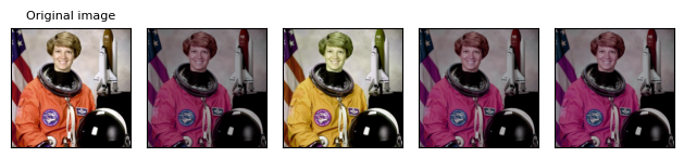
Fig 7. Color Jitter Example [4].
The Models
Deep learning has become one of the most popular tools for computer vision and machine learning ever since our computation power increased to the level required to take in the massive amounts of data these models require. Deep Learning models are in a sense exactly how they sound. They are neural networks with many many layers to capture different aspects of data features using backpropogation and series of linear and non-linear transformations to update the learning parameters. We are using several baseline pretrained models with altered output layers for comparison. We extracted the best possible accuracy from Resnet18, Resnet50, VGG16, and ViT with our data. Our goal is to use an ensemble of these different models to try and compensate for our limited dataset, but this goal is gated behind training speed.
Ensemble
Individual deep learning networks can be extremely successful at classifying difficult data. How much more so then can a group of these models predict the data together. This is the idea behind an ensemble of models. Each model makes a classification and takes the majority vote betwwen them as the final classification. However, the accuracy of the models we have trained are very different so the regular majority vote did not out achieve our best model by itself. To make up for this imbalance, we can instead do a weighted ensemble where certain models have a stronger vote. We decided to weigh the models by their accuracy with our best model having the highest weight in the vote for the final classification.
ViT
Vision Transformers (ViT) are another model for image recognition that take in an input image as a series of image tokens. They take in each token combined with a positional encoding. This gives the model some initial notion of where the tokens are in relation with one another since they are not just in sequential order like some NLP data that is used in transformers. From here, attention weights are learned between one token to all of the others for each individual token. These attention weights can extract global relationships from the data that can be difficult to get from simple sequential input because they detail the relation between tokens. i.e. how important is this token in the context of another (such as the word he specifically representing to the name Thomas in the sentence “Thomas met a girl named Lucy and he fell in love.”). After the multi-head self attention layer residual connections reinput the original token embeddings onto the learned embeddings to complete the pass through the network without passing through any non-linear activations. This process can outperform CNN’s significantly in efficiency as pixel arrays and stacked layers of activation functions and convolution are not needed.
Self-Attention
Self attention is what ViT’s use as their primary learning method. The process begins with an embedding of our token x (token and positional embedding) which is multiplied with three matrices of parameters to produce three vectors called Query, Key, and Value (Q,V,K). The Q vector of the input token we are working on is multiplied with the key of each of the other tokens in te input giving a score for each that represents their weighted importance to the current token. Then they are divided by the square root of the dimension of k for normalization and are put through softmax to become probability values. Then, they are finally multiplied with the value vector and put together in a weighted sum to get the final attention vector.
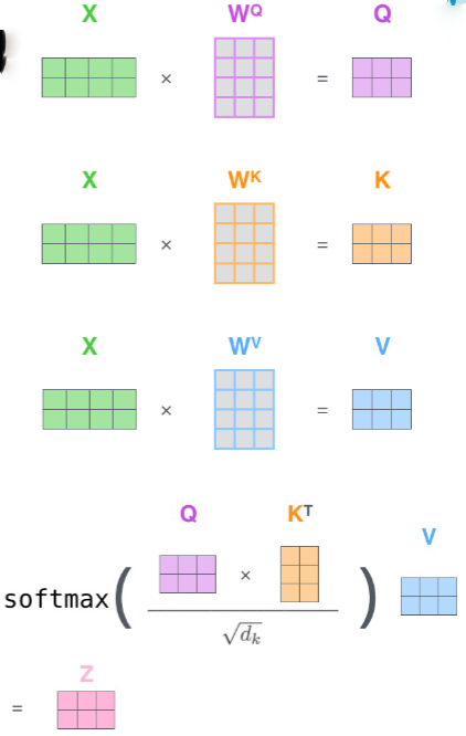
Fig 8. Self-Attention Mechanism courtesy of Violet Peng CS162
Training ViT
Initial attempts to train ViT with SGD, a learning rate of 0.01, and momentum of 0.9 were dismal; nearly no learning occurred. We learned that this is because Adam imperically far outperforms SGD for training ViT. After switching to Adam with a learning rate of 0.004, we had much better performance.
VGG
In 2012, AlexNet shocked the world with its eight layer net, which was deeper than any of its competition at the time. Its successor is called VGGNet, produced by the Visual Geometry Group at Oxford (Somonyan 2015). VGG comes in 16 or 19 layers, and it achieved this increase in the number of layers with one innovation: they set the filter size to 3x3 for every convolutional layer. We use Pytorch’s vgg16, which has 16 layers and is pretrained on ImageNet1K. The researchers found that deeper versions of vgg suffered from the vanishing gradients problem.
Training VGG
VGG trains very slowly; our initial tests were running at 17 seconds per iteration on a premium colab GPU. In an effort to reduce the training time for each epoch, we downsampled the dataset to a third of its original size and then froze all of the convolutional layers. Our goal was to train only the fully connected layers, thus using the initially pretrained convolutional layers as a feature extractor. Eventually we were able to reach a reasonable training time of 20 minutes per epoch.
We trained VGG using Momentum SGD with a learning rate of 0.01 and momentum of 0.9. These hyperparameters definitely need tuning, as learning stops after the first epoch. We unfortunately did not have the resources to do hyperparameter tuning through Ray Tune, which would have allowed us to select the best learning rate. It might also have been better to use Adam, although the relative benefits could only be found imperically.
ResNet
In theory, deeper nets would result in better performance, but deep learning nets encountered one big problem: vanishing gradients. Researchers found that if neural nets were deep, their gradients would fail to propagate through the layers. This changed in 2015 with the introduction of the Residual Net and its innovation of the residual by Kaiming He (He 2015). ResNet uses residuals to allow layer inputs to bypass each layer so that the input to the system directly impacts every single layer. Consequently, the gradient of the output directly affects every layer as well, enabling gradients to propagate all the way through the system. We used two pretrained implementations of Kaiming’s original paper through Pytorch’s ResNet18 and ResNet50. These models each contain many residual convolutional layers, one MaxPool layer, and one average pool layer. Additionally, the models have a fully connected layer at the end so that they can be used for classification. They have both been pretrained on ImageNet1K.
Training Resnet
ResNet, when trained on our entire augmented dataset with SGD, a learning rate of 0.01, and a momentum of 0.9, trained far faster than our other models. Consequently, we were able to train it for more epochs given our resources.
Results
We were limited by our training resources; our training rate was approximately one epoch every forty minutes using a premium Google Colab GPU. Therefore, in order to conserve resources, we trained each of our models for 5 epochs. Clearly, for all of our models, this was far from enough. Our models had consistent validation accuracy increases after every epoch. Resnet18 had inconsistent accuracy increases of around 4 percent accuracy, starting at 11 percent and ending at 24 percent accuracy. Resnet50 saw close to ten percent increases in validation accuracy after almost every epoch. Our initial accuracy was 31 percent, and our final accuracy was 64 percent. We encountered an abnormality where our accuracy actually dropped after the fourth epoch, but then it resumed climbing after the fifth epoch, as seen in Figure 9. We expect that if we had more training time, we could have achieved much higher validation accuracy. In contrast to Resnet, VGG was less impressive. We saw approximately 3 percent improvements after each epoch consistently over training, starting at 12 percent and ending at 24 percent. Once again, we expect that our model would have improved with more training time. VGG was extremely slow to train, possibly because of the large numbers of parameters in its fully connected output layers, so we had to train it on a reduced dataset without all of our data augmentation in order to keep the training time for each epoch under an hour. In contrast, our attempts at ViT were dismal. It began with 2 percent validation accuracy and increased consistently but slowly to 13 percent over the course of training. We know that transformers require more training time and larger datasets, and we learned in our homework that they perform poorly on short training. When we attempted to use all four models in an ensemble, we were limited by their varied performances, and we were unable to get a higher validation accuracy than 64 percent, which was the accuracy of Resnet. We believe that with 1394 categories to choose from, the four models picked four separate labels on the majority of occasions; our ensemble model’s accuracy effectively became the accuracy of whatever model we used for tiebreaking in the case of a four-way tie. Because our ViT model had such poor performance, it nearly never aligned with VGG or Resnet18 to outvote ResNet50 when ResNet50 was incorrect. If Resnet50 was our tiebreaker, then the ensemble model had a slightly lower validation accuracy to Resnet alone. If either of the other models was the tiebreaker, then our performance aligned with that model and fell somewhere between that model’s performance and ResNet’s performance. We then implemented a weighted ensemble and, as expected, encountered a similar problem; our performance was best when Resnet50 had a very high weight so that it could outvote the others. We were not able to achieve an accuracy above Resnet50’s accuracy of 64 percent.
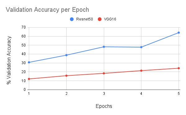
Fig 9. Validation Accuracy per Epoch for VGG16 and Resnet50
Conclusion
Although we were unable to use our ensemble to improve our performance, we learned a different lesson about the importance of training resources when working with big data sets.
Our idea behind the ensemble model was that we would hit an upper bound on the validation accuracy of our models relatively quickly and then need to construct other models in parallel to continue to improve performance. As it turned out, our problem was very different: ae simply were unable to train any of our models for long enough to optimize our accuracy – up until the very last epoch, they were still improving without slowing down in any way. And yet, even without optimizing to the fullest, we had a shockingly high accuracy on Resnet50 of 64% accuracy. When initially approaching this project, we saw that the top scorers in the Kaggle competition achieved accuracies in the high eighties and mid nineties for their submissions; these submissions came from big teams with lots of training resources. In contrast, our group consists of two students who could only train on a single GPU for as long as we could keep a Google Colab instance open. The fact that we were able to achieve 64 percent validation accuracy on this huge and complex dataset is a testament to the power of pretrained models.
Before we remembered to use pretrained weights, we accidentally trained Resnet50 for a few epochs from scratch with default weights. We had accuracies in the range of 10 to 20 percent after multiple epochs, but with the introduction of pretrained weights we were able to increase our accuracy after a single epoch to 31 percent. Resnet50’s pretrained weights came from a huge amount of training done on ImageNet images; in order to do the same amount of training on our own, we would have needed to spend thousands of dollars in compute time, but it is offered to everyone for free on Pytorch. We learned that open source pretrained models enable anyone with a computer to achieve impressive classification accuracies with minimal computing power, which explains how the industry is advancing so quickly; if it is so cheap, fast, and easy to apply a powerful pretrained model to a problem, then soon deep learning models will be everywhere.
Code Repositories
[0] 2018 FGVCx Competition Dataset and Repository
References
[1] Mushrooms Detection, Localization and 3D Pose Estimation…. Baisa, Nathanael L., and Bashir Al-Diri. Mushrooms Detection, Localization and 3D Pose Estimation Using RGB-D Sensor for Robotic-Picking Applications. Arxiv, 8 Jan. 2022, https://arxiv.org/pdf/2201.02837.pdf.
[2] Mohanty, Sharada P., et al. “Using Deep Learning for Image-Based Plant Disease Detection.” Frontiers, Frontiers, 6 Sept. 2016, https://www.frontiersin.org/articles/10.3389/fpls.2016.01419/full.
[3] N, Skanda H. Plant Identification Methodologies Using Machine Learning … - IJERT. Https://Www.ijert.org/, 3 Mar. 2019, https://www.ijert.org/research/plant-identification-methodologies-using-machine-learning-algorithms-IJERTV8IS030116.pdf.
[4] “Transforming and Augmenting Images¶.” Transforming and Augmenting Images - Torchvision Main Documentation, https://pytorch.org/vision/master/transforms.html.
[5] He, Kaiming., et al. “Deep Residual Learning for Image Recognition.” CoRR, 10 Dec 2015. https://arxiv.org/abs/1512.03385
[6] Somonyan, Karen and Zisserman, Andrew. “Very Deep Convolutional Networks for Large-Scale Image Recognition.” University of Oxford. ICLR 2015. https://arxiv.org/pdf/1409.1556.pdf