This project focuses on the generating images from text using diffusion models.

• TOC

Fine-tuning stable diffusion using textual inversion

Before we discuss stable diffusion in more details, we need to establish a few fundamental tools that are used by the model.

Autoencoders

In order to motivate the need for autoencoders, we first study the problem of dimensionality reduction which is the process of reducing the number of features describing data. Dimensionality reduction can be performed by selecting certain features or extracting a new set of features from our original features. 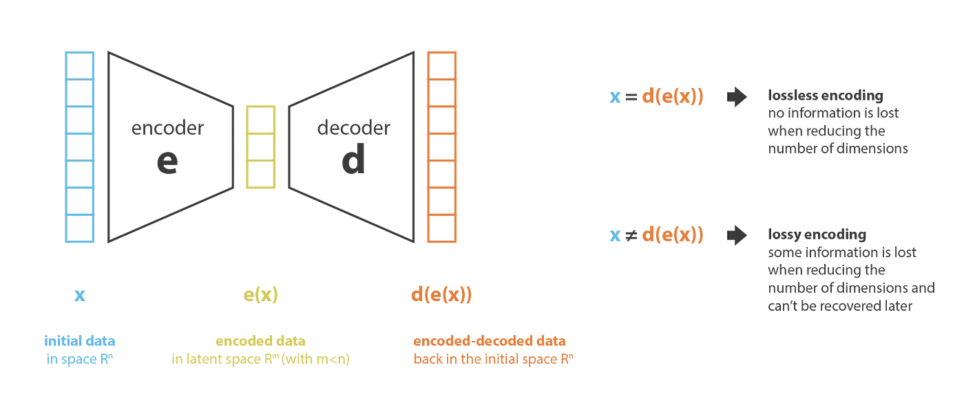An autoencoder consists of an encoder and a decoder. The encoder produces new features in a lower dimensional space than the original features. The encoder therefore compresses the data from the initial space into the latent space. Conversely, the decoder decompresses the data from the latent space back to the original space. The compression is generally lossy which means that some data cannot be recovered by decoding. Our goal is to find the best encoder/decoder pair, which is an encoder/decoder that keeps the maximum amount of information while encoding and has the minimum amount of information lost during decoding. If $E$ and $D$ are families of encoders and decoders respectively, the dimensionality reduction problem can be mathematically expressed in the form \((e^*, d^*) = \argmin_{(e, d) \in E \times D} \epsilon(x, d(e(x)))\) where $\epsilon(x, d(e(x)))$ is the reconstruction error between the input data and the encoded-decoded data. In an autoencoder, we set the encoder and decoder to be neural networks. Let $x$ represent the input data, $z = e(x)$ represent the latent representation of $x$ created using encoder $e$ and $\hat{x} = d(z)$ be the result of running decoder $d$ on the latent representation $z$. The loss is then calculated to be \(\| x - \bar{x} \|^2 = \| x - d(z) \|^2 = \| x - d(e(x)) \|^2\)

We then learn the best encoder and decoder using backpropogation and gradient descent. [1]

Variational Autoencoders

One major weakness of autoencoders is that lossless dimensionality reduction often leads to a lack of regularity in the latent space. One of the primary goals of dimensionality reduction is to reduce the number of dimensions while simultaneously maintaining structure that exists in the data in the original representation. Variational autoencoders are autoencoders that have their encoding distributions regularized during training to prevent overfitting, which helps ensure that the latent space has a desirable structure and can be sampled to produce new data. In order to do this, a variational autoencoder encodes each input as a distribution over the latent space instead of as a single point. In order to train the model input is first encoded as a distribution over the latent space. Next, a point from the latent space is sampled from the distribution. The sampled point is decoded and the reconstruction error is computed. Finally, the reconstruction error is backpropagated through the network. The encoded distributions are generally chosen to be normal so that the encoder can be trained to return the mean and covariance matrix describing the distributions. The benefit of encoding an input as a distribution is that it greatly simplifies the regularization process since the distributions returned by the encoder can be forced to be close to a normal distribution. Some methods that are used to force the distribution to be close to a normal distribution are explained later while taking a closer look at diffusion and latent diffusion models.

Diffusion Models

Diffusion models represent the state-of-the-art approach for image generation. These are based on the concept of diffusion in thermodynamics, in which structure is destroyed over time as particles move from high to low concentration. In the context of image generation, the model pipeline involves two steps: the forward process and reverse process. In the forward process, the input image is repeatedly augmented with Gaussian noise. The model is trained to accurately estimate the noise added to the image. In the reverse process, the model takes a random image and subtracts the predicted noise, generating a new image based on the predictions.

Forward Process

The forward process involves the repeated application of a Markov chain, or a sequence of events in which the probability of each event depends only on the state attained by its predecessor.

More concretely, given an initial data distribution $q(x_0)$, the distribution at time $t$ depends only on the addition of Gaussian noise to the distribution at time $t-1$:

\[q(\mathbf{x}_t|\mathbf{x}_{x-1}) = \mathcal{N}(\mathbf{x}_t; \mathbf{x}_{t−1}\sqrt{1 − \beta_t},\mathbf{I}\beta_t)\]

$\beta_0$ is the standard deviation of each dimension of the distribution, or the diffusion rate, and is tunable as a hyperparameter [2].

An initial analysis of this approach seems to suggest that the above calculation must be repeated $t$ times to obtain the distribution at time $t$, making the process very inefficient. However, through the use of the reparameterization trick, it is possible to perform closed-form sampling at any timestamp.

Let $\alpha_t = 1-\beta_t$, and $\bar{\alpha}t = \prod{s=0}^{t}\alpha_s$. Given $\bm{\epsilon},…,\bm{\epsilon}_{t-1}, \bm{\epsilon}_t \sim \mathcal{N}(\mathbf{0},\mathbf{I})$:

\[\mathbf{x}_t \sim q(\mathbf{x}_t|\mathbf{x}_0) = \mathcal{N}(\mathbf{x}_t; \sqrt{\bar{\alpha}_t}\mathbf{x}_0,(1 - \bar{\alpha}_t)\mathbf{I})\]

Since $\beta_0$ is a hyperparameter, all $\bar{\alpha}_t$ can be precomputed, allowing $\mathbf{x}$ to be sampled at any arbitrary $t$ [3].

Reverse Process

As $t \rightarrow \infty$, $\mathbf{x}t \rightarrow \mathcal{N}(0,\mathbf{I})$. The reverse process takes an input from $q(\mathbf{x}_t)$ and producing a sample from $q(\mathbf{x}_0)$ by applying the reverse distribution $q(\mathbf{x}{t-1}

\mathbf{x}_t)$.

Unfortunately, computing this distribution is intractable, and so a neural network is instead used to approximate it. The learned distribution will be designated $p_\theta(\mathbf{x})$ Formulating the reverse process as a Markov chain produces the following expression for $p_\theta(\mathbf{x}_0)$:

\[p_\theta(\mathbf{x}_0) = p_\theta(\mathbf{x}_t)\prod_{t=1}^Tp_\theta(\mathbf{x}_{t-1}|\mathbf{x}_t)\]

The neural network can then learn the mean $\mu_\theta(\mathbf{x}t,t)$ and the variance $\sigma\theta(\mathbf{x}_t,t)$ for the distribution at each time $t$ [3].

Training the Model

As is common in machine learning, this model can be optimized by maximizing the negative log-likelihood on the training data. However, once again this calculation is intractable. Instead, the negative log-likelihood has a lower bound as follows:

\[logp(\mathbf{x}) \ge \mathbb{E}_q(x_1|x_0)[logp_\theta(\mathbf{x}_0|\mathbf{x}_1)]- \\ D_{KL}(q(\mathbf{x}_T|\mathbf{x}_0)||p(\mathbf{x_T})) - \\ \sum_{t=2}^T\mathbb{E}_q(x_t|x_0)[D_{KL}(q(x_{t-1}|\mathbf{x}_t,\mathbf{x}_0)||p_\theta(\mathbf{x}_{t-1}|\mathbf{x}_t))]\]

Here $D_{KL}$ is the Kullback-Leibler divergence, which measures the difference between two indicated distributions. This formulation is known as the evidence lower bound (ELBO).

Of relevance to the neural network is the third term above, which contains the summations of all KL divergences between the correct denoising steps and the learned ones. Maximizing the similarities between these distributions will minimize the KL-divergence and thus maximize the ELBO [3].

Once again, using the reparameterization trick (with the same definition of $\alpha$ and $\bar{\alpha}$), the target mean $\tilde{\mu}$ can be expressed as follows:

\[\tilde{\mu}_\theta (\mathbf{x}_t,t) = \dfrac{1}{\sqrt{\alpha_t}} \left(\mathbf{x}_t - \dfrac{\beta_t}{\sqrt{1-\bar{\alpha}_t}}\bm{\epsilon}_\theta(\mathbf{x}_t,t) \right)\]

Thus, the third term in the ELBO can be expressed as follows:

\[\mathbb{E}_{\mathbf{x}_0,t,\bm{\epsilon}} \left[\frac{\beta_t^2}{2\alpha_t(1-\bar{\alpha}_t)||\mathbf{\Sigma}_\theta||_2^2}||\bm{\epsilon}_t-\bm{\epsilon}_\theta(\sqrt{\bar{\alpha_t}}\mathbf{x}_0+\sqrt{1-\bar{\alpha}_t}\epsilon,t)||^2 \right]\]

The model predicts the noise $\epsilon_t$ for each $t$.

Latent Diffusion Models

Traditional diffusion models typically operate in pixel space and so consume a large number of GPU days. Therefore, inference is expensive as a result of the large number of sequential evaluations. Latent diffusion models help enable diffusion model training using limited computational resources without significantly altering the quality of the result by applying diffusion models in a latent space generated using autoencoders. The process of generating this latent space is known as perceptual image compression.

Diffusion models are extremely costly to train as they require function evaluations in pixel space. In order to circumvent this problem, latent diffusion models use an autoencoding model which learns a space that is roughly equivalent to pixel space but has a far lower dimensionality and therefore allows training to be far more efficient. Further, the process produces general-purpose compression models whose latent space can be used to train other generative models. An existing autoencoder architecture was used that was specifically designed to enforce local realism and avoid blurriness. In latent diffusion, the autoencoder consists of an encoder $\epsilon$ and a decoder $\mathcal{D}$ that encodes an image $x \in \mathbb{R}^{H \times W \times 3}$ in RGB-space into a latent representation $z = \epsilon(x)$ and the decoder reconstructs the image from the latent form and computes $\bar{x} = \mathcal{D}(z) = D(\epsilon(x))$, where $z \in R^{h \times w \times c}$. The encoder therefore downsamples the image by a factor of $f = H/h = W/w$. The autoencoder thus tries to train an encoder and decoder to ensure that the original image is decoded as accurately as possible. The lower-dimensional space produced using perceptual image compression is more suited to likelihood-based generative models since it is better able to focus on important portions of the data and train in a lower dimensional and hence more computationally efficient space.

In order to limit the variance of latent stages produced by the autoencoder, two models were trained using KL regularization and VQ regularization. These two forms of regularization are discussed below.

KL Regularization

The first type of regularization used is known as KL-reg which attempts to ensure the latent representation is similar to a normal distribution. KL Regularization uses an idea known as KL divergence which measures the difference between two probability distributions. When two distributions are identical, the KL Divergence between them is 0. The KL divergence is computed to be \(D_{KL} (P || Q) = \sum\limits_{x \in X} P(x) \left[ \log \frac{P(X)}{Q(X)} \right]\) where $X$ is the probability space. [4] We breakdown the above formula to better understand it. When the probability $Q(x)$ is higher than $P(X)$, this component of the formula produces a negative value. Conversely, if $Q(x)$ is always smaller than $P(x)$, the component produces positive values. We multiply the logarithmic term by $P(x)$ to make it an expected value.

VQ Regularization

The second regularization method is called VQ-req. VQ-regularization is used in a special type of variational autoencoder that enables VAEs to mitigate issues of posterior collapse, which is when latents are ignored when they are paired with a powerful autoregressive decoder. A diagram for VQ-VAEs is provided below. As observed in the diagram, we take a vector in latent space and find the closest vector to it according to the L2-norm in the codebook, which is represented by the purple blocks labeled $e_i$. We then index into the codebook to extract discrete latent vectors which are fed into the decoder to produce an image. We therefore observe that the VQ-VAEs operate on a discrete latent space rather than a continuous latent space. This makes optimization far more efficient since it is much easier to learn distributions in the discrete latent space than in a continuous latent space. [5]

Architecture

As discussed above, in a latent diffusion model the objective can be written as

\[L_{DM} = \mathbb{E}_{x, \epsilon \sim \mathcal{N}(0, 1), t} \left[ || \epsilon - \epsilon_{\theta} (x_t, t) ||_2^2 \right].\]

In latent diffusion, our objective can now be written as

\[L_{LDM} := \mathbb{E}_{\varepsilon(x), \epsilon \sim \mathcal{N}(0, 1), t} \left[ || \epsilon - \epsilon_{\theta} (z_t, t) ||_2^2 \right]\]

The latent representation provides an efficient low-dimensional space that eliminates redundant high-frequency details. The latent diffusion model architecture is therefore able to exploit image-specific inductive biases from the latent space. The architecture for latent diffusion models is provided below. 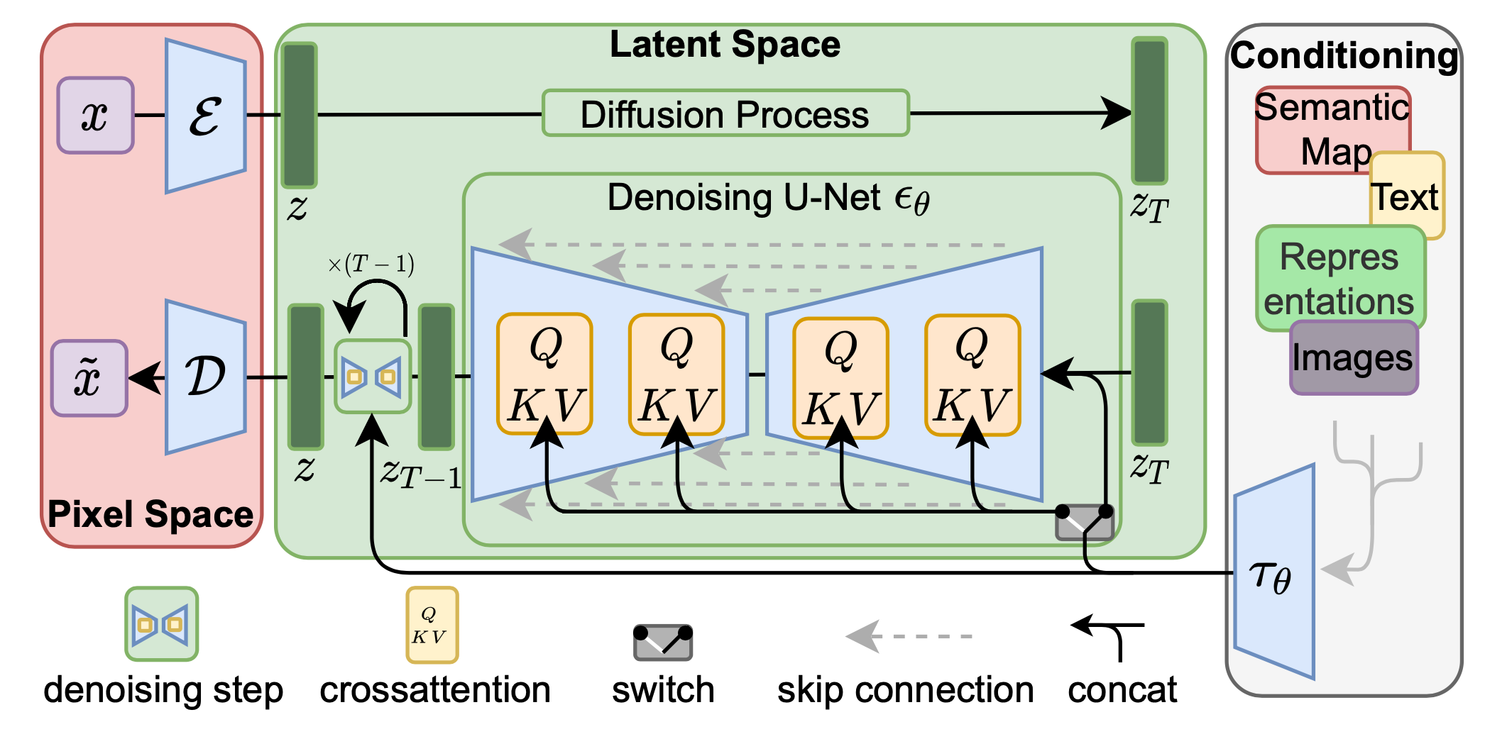As seen in the diagram, the diffusion and denoising process happen on the vector $z$ in latent space. The model can accept different types of inputs such as text, semantic maps, images and representations. The input is processed to produce conditioning information for image generation and input into the model using $\tau_\theta$. The preprocessing differs based on the type of the input.

The diffusion process is demonstrated in the bottom of the diagram. The neural backbone of the model is the neural network U-net. The model is augmented with a cross-attention mechanism that enables it to utilize flexible conditioning information from $\tau_\theta$. Then attention is computed to be \(\operatorname{Attention}(Q, K, V) = \operatorname{softmax}\left( \frac{QK^T}{\sqrt{d}} \right) \cdot v\) where \(Q = W_Q^{(i)} \cdot \varphi_i(z_t),\, K = W_k^{(i)} \cdot \tau_{\theta}(y), V = W_V^{(i)} \cdot \tau_{\theta}(y).\) In the above formula, $\varphi_i(z_t) \in \mathbb{R}^{N \times d_{\epsilon}^i}$ is used to represent a flattened intermediate representation of the U-net implementing $\epsilon_{\theta}$ and $W_v^{(i)} \in \mathbb{R}^{d \times d^i_{\epsilon}}, W_Q^{(i)} \in \mathbb{R}^{d \times d_{\tau}}$ and $W_k^{(i)} \in \mathbb{R}^{d \times d_{\tau}}$ are learnable projection matrices.

Using the image conditioning pairs, we now learn \(L_{LDM} := \mathbb{E}_{\varepsilon(x), y, \epsilon \sim \mathcal{N}(0, 1), t} \left[ || \epsilon - \epsilon_{\theta} (z_t, t, \tau_\theta (y)) ||_2^2 \right]\) where $\tau_\theta$ and $\epsilon_\theta$ are jointly optimized using the above equation [6].

Fine-tuning stable diffusion using textual inversion

Textual inversion is a technique used to learn novel concepts from a small number of example images that can then be used in text to image pipelines. The model therefore learns new words in the embedding space of the pipeline’s text encoder. The added words can then be used in text prompts to generate new images based on the training images. 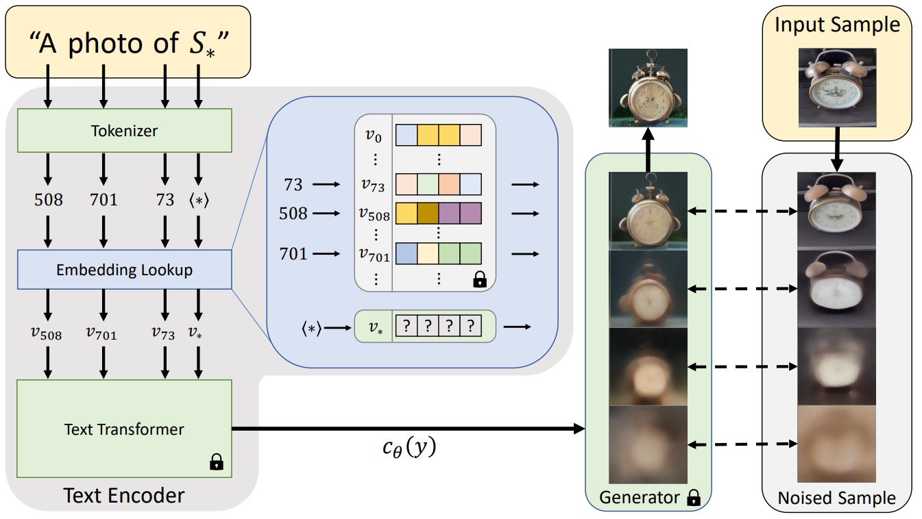Any text prompt passed in is first tokenized into a numerical representation that converts each token into an embedding that is fed through a transformer whose output is used to condition the diffusion model. After fine-tuning using textual inversion, the model learns a new embedding (represented by $v^*$ in in the diagram above). A token is mapped to this new embedding and is used together with a diffusion model in order to predict a denoised version of the image. The model is trained and the embedding is improved to better capture the object or style present in the training images and can therefore be used to generate images that utilize the new token that has been learnt.

Method

Our code was based heavily off of the work in the following google collaboratory notebook: https://huggingface.co/docs/diffusers/training/text_inversion. A link to our code is https://colab.research.google.com/drive/121-zeCUnTE2uchMMa6svERFr_B4HYdEo?usp=sharing

The goal of this process is to produce images featuring UCLA mascot Joe Bruin.

Environment Setup

The first step of the process was to find training images that would eventually be used to perform textual inversion. For this purpose, four images of UCLA mascot Joe Bruin were found across UCLA’s website, padded into square images using Square my Image, and uploaded to Imgur for consistent access.

Additionally, Hugging Face can optionally be utilized to store the binaries associated with the newly learned model in the concept library. Doing so requires creating a Hugging Face account and generating an access token with write permissions.

Pipeline

The training process is based on the Stable Diffusion 2 model.

The first step is to define three parameters that will identify the training concept: what_to_teach (either ‘object’ or ‘style’ depending on the type of training), placeholder_token (a representative token for the new concept within the prompt), and initializer_token (a hint to the model to serve as a starting point for the new concept). The values for these three parameters are “object”, “<joe-bruin>”, and “bear” respectively. A training dataset is generated using a set of prompt templates and the training images.

Next, the tokenizer of the diffusion model is augmented with the placeholder token. Now only the embedding associated with the new token needs to be learned during training time, so the rest of the model parameters are frozen.

With the model initialized, it is run for 2000 iterations at a learning rate of .0005.

Results

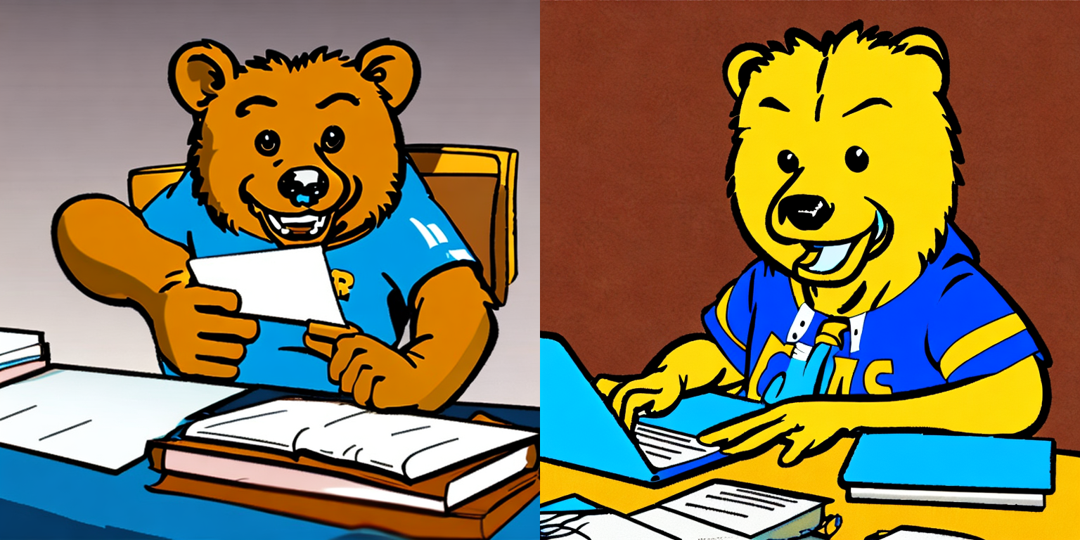
Prompt: “<joe-bruin> doing homework”

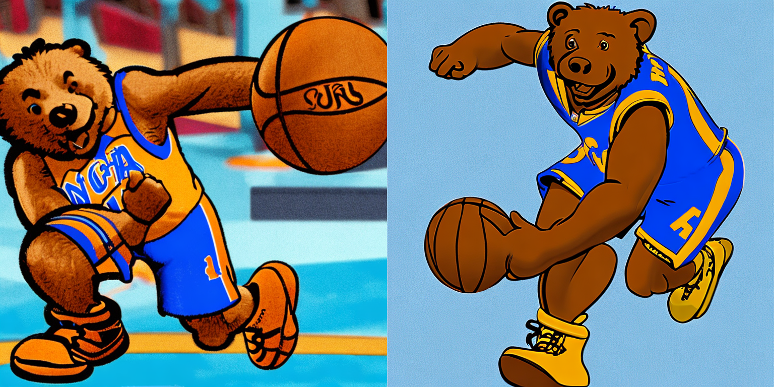
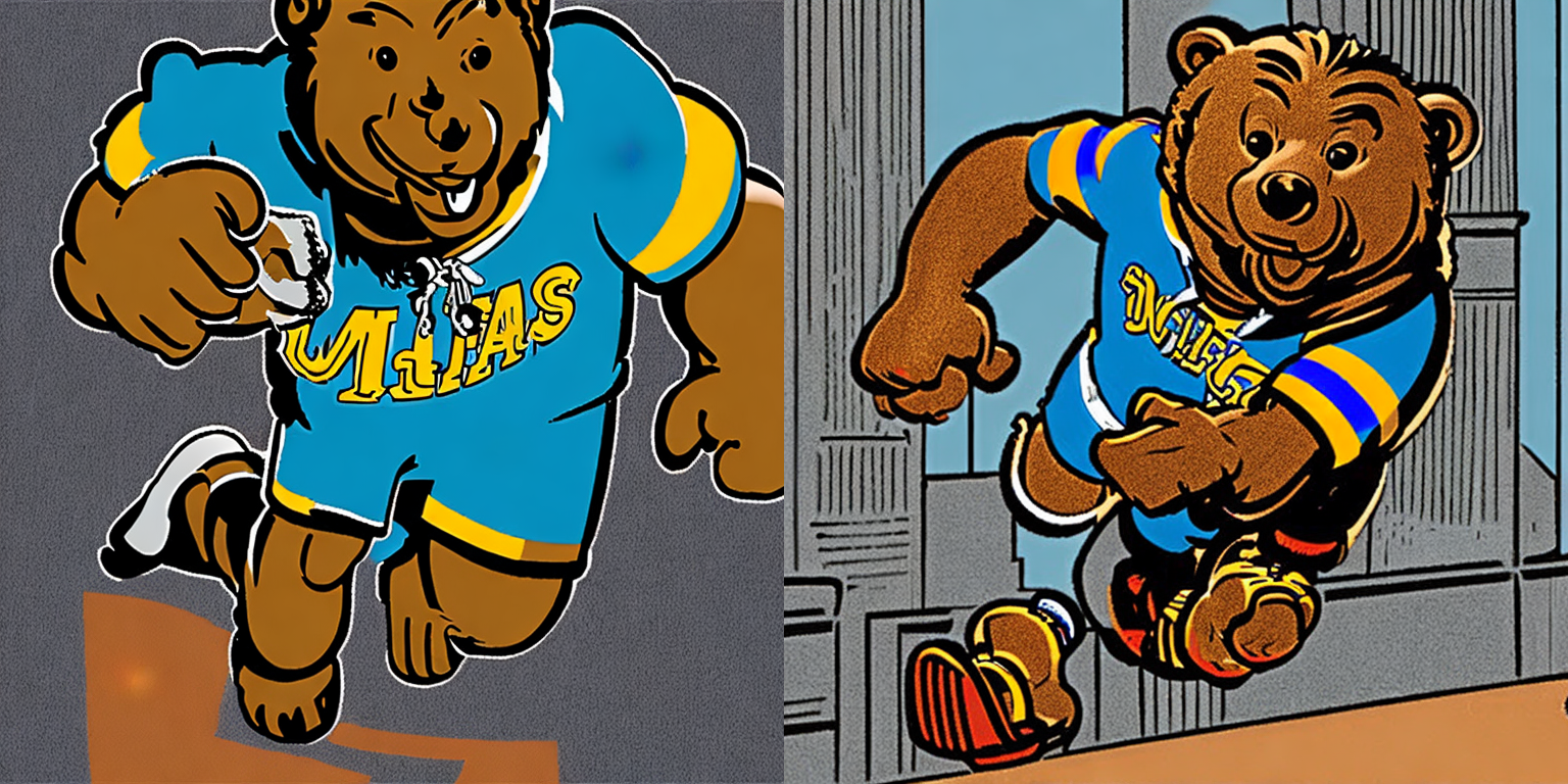
Prompt: “<joe-bruin> playing basketball”

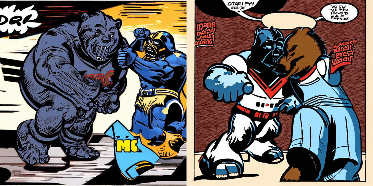
Prompt: “<joe-bruin> fighting darth vader”

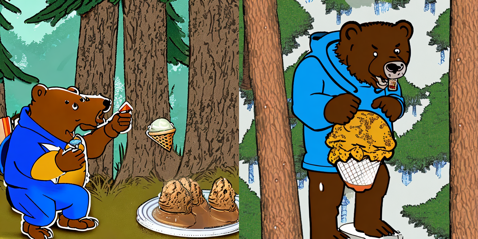
Prompt: “<joe-bruin> eating ice cream in the woods”

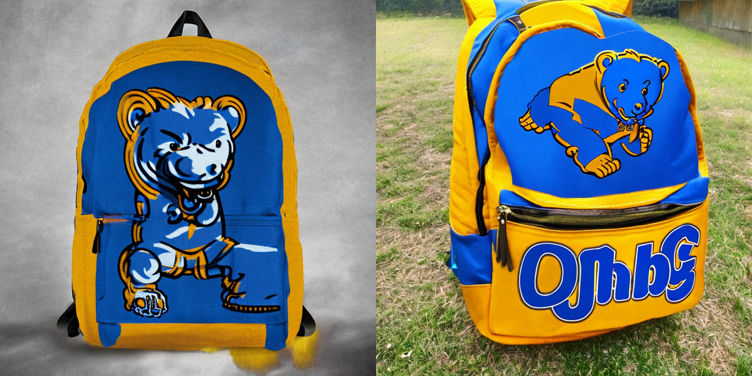
Prompt: “backpack showing <joe-bruin>”

Prompt: “a man riding <joe-bruin>”

Discussion

As evidenced by the results displayed above, given simple prompts that the model has apparent familiarity with, the outputs reasonably match the prompts. The former 4 results use <joe-bruin> as the subject of the prompt and contain only simple additional qualifiers; these all produce high-quality results. However, last 2 results change the structure of the prompt, either using abstract adjectives to modify <joe-bruin> or using the token as the object of the phrase. These results were much more inconsistent, suggesting that the model lacked familiarity with these more complex structures. Resolving such a gap may require further augmentation of the training dataset with additional prompts to produce better results.

Video Demo

References

[1] Rocca, Joseph. “Understanding Variational Autoencoders (VAES).” Medium, Towards Data Science, 21 Mar. 2021, https://towardsdatascience.com/understanding-variational-autoencoders-vaes-f70510919f73.

[2] Sohl-Dickstein, Jascha, et al. “Deep Unsupervised Learning Using Nonequilibrium Thermodynamics.” Arvix, 12 Mar. 2015.

[3] Karagiannakos, Sergios and Nikolas Adaloglou. “How Diffusion Models Work: The Math from Scratch.” AI Summer, Sergios Karagiannakos, 29 Sept. 2022, https://theaisummer.com/diffusion-models/.

[4] Rath, Sovit Ranjan. “Sparse Autoencoders Using KL Divergence with Pytorch.” DebuggerCafe, 30 Mar. 2020, https://debuggercafe.com/sparse-autoencoders-using-kl-divergence-with-pytorch/.

[5] Oord, Aaron van den, et al. “Neural Discrete Representation Learning.” Arvix, 2 Nov. 2017.

[6] Rombach, Robin, et al. “High-Resolution Image Synthesis with Latent Diffusion Models.” 2022 IEEE/CVF Conference on Computer Vision and Pattern Recognition (CVPR), 2022, https://doi.org/10.1109/cvpr52688.2022.01042.