Mitigating Spurious Correlations in Deep Learning
Spurious correlations pose a major challenge in training deep learning models that can generalize well to arbitrary real life data. Models often exploit easy-to-learn features that are correlated with prediction(s) in the training set but not semantically meaningful in the real world. In this post, we provide an overview of the spurious correlation problem by characterizing it mathematically, discuss some of its causes, and describe three key methods for mitigating such correlations: GroupDRO, GEORGE, and SPARE, along with some empirical results for each method.
- Introduction to Spurious Correlations
- Deeper Characterization of Spurious Correlations
- Causes of Spurious Correlations
- Methods for Mitigating Spurious Correlations
- Experiments
- Tradeoffs when Dealing with Spurious Correlations
- Conclusion
- References
Introduction to Spurious Correlations
Deep neural networks have achieved remarkable success across a wide range of tasks. However, they often rely on superficial correlations between input features and labels that do not reflect a meaningful relationship. For example, in a dataset of images of cows and camels, the model may learn to associate “cow” with green pastures and “camel” with sandy deserts, rather than learning the relevant semantic features of the animals themselves. As a result, the model may fail to generalize to cows in deserts or camels in pastures, an obvious bias. This sort of problem is known as a spurious correlation. In general, a model learns spurious correlations when it begins to associate certain features with prediction(s), when those features are not truly related to the prediction, i.e. in the camel/cow example.
Deeper Characterization of Spurious Correlations
Conventional Optimization Objective (ERM)
We begin by providing a mathematical overview of the conventional optimization objective used to train the models in question. The particular method used is known as Empirical Risk Minimization (ERM). The canonical equation for ERM is given below.
\[w^* \in \text{arg min}_w \mathbb{E}_{(x_i,y_i) \in \mathcal{D}} [\ell(f(w, x_i), y_i)],\]Where each symbol is defined as follows.
- \(w^*\): The optimal weights or parameters for our model. We attempt to find the best possible values for these weights that minimize the loss over our training dataset.
- \(\text{arg min}_w\): The set of values \(w\) which minimize the following expectation.
- \(\mathcal{D}\): The data distribution from which our data points \((x_i, y_i)\) are drawn. In practice, this is often the empirical distribution defined by our available dataset.
- \(\ell\): A loss function that measures the discrepancy between the predicted values \(f(w, x_i)\) and the actual labels \(y_i\) (commonly a cross entropy loss in the case of multiple classification).
- \(f(w, x_i)\): Our model’s prediction, with weights \(w\) and input features \(x_i\).
The goal of the optimization problem described by this equation is to find the best parameters \(w\) that lead to the smallest possible average loss on our data. By doing so, we train a model that is, hopefully, both accurate and generalizable.
However, in the presence of spurious correlations, ERM may learn to rely on the simple spurious features to minimize the average loss. This results in poor worst-group performance, i.e., high error on the group where the spurious correlation does not hold. A few example cases of this are given in the next section.
Examples of Spurious Correlations
Some common examples of spurious correlations include:
Object recognition: The background (e.g., grassy, sandy, watery) may be spuriously correlated with the object class (e.g., cow, camel, waterbird), when the background is not truly a core feature determining the nature of the animal in the input image.
Natural language inference: The presence of certain words (e.g., “not”, “no”) may be spuriously correlated with the contradiction label, even when this might not be the case.
As a more concrete example, see:
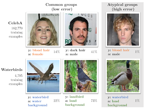
Fig 1. Examples of Spuriously Correlated Features in Two Separate Contexts [4].
Consider the top row of this image. In the training dataset, we have a that images of females with blonde hair are common, as are images of males with dark hair. However, for example, images of males with blonde hair are rare. Thus, if we train a model to classify the gender of a person given an image of their face using the following dataset, the model will likely have significantly higher error rates on atypical groups (e.g. males with blonde hair here). This is an example of a spuriously correlated feature, where the core feature is male/female, and the spurious feature is the hair color (which we trivially know to not determine the gender of a person).
A similar situation is present in the second row of the image. In this case, we are concerned with classifying landbirds vs. waterbirds (core feature). Within the dataset, landbirds are often pictured with land (green, grassy, foliage) in the background, and waterbirds are often pictured with water in the background. However, we know that the background of the image does not determine what type of bird is necessarily present (we can have waterbirds on land and vice versa). Thus, a model trained on this dataset to classify the core feature of land/water bird may learn the spurious correlation between the background and the type of bird in the image. This may lead to lower performance on atypical groups (waterbirds on land, or landbirds in water).
This interpretation of a model potentially highly weighing a spurious feature when performing classification is also supported by a Grad-CAM heatmap of the model’s outputs given various images:
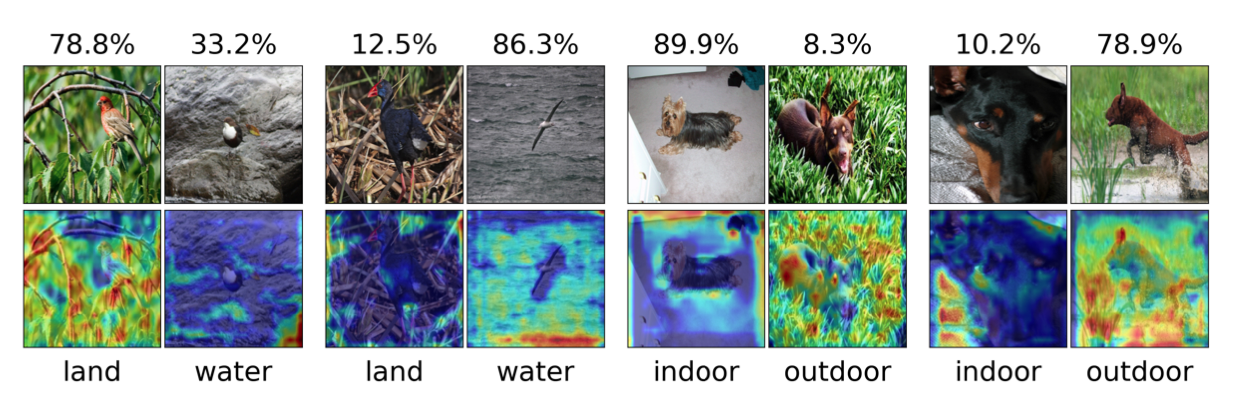
Fig 2. Grad-CAM heatmaps of model(s) which have learned spurious features. [2].
The above heatmaps support this intuition. We see much higher weights being placed on the backgrounds of the images vs the actual subject (which is the object to be classified in both cases). The fourth image from the left demonstrates the spurious correlation exactly. We see the model highly weighing most of the pixels in the background and explicitly not taking into account the region where the bird is in the image. This same phenomenon occurs in the other images as well, with the model placing a significant weight on the background (which we want to be relatively unrelated to model output). Thus, these activation mappings go to show the nature of a model which has learned spurious correlations.
Spurious Correlation Key Metric (Worst-Group Test Error)
To address spurious correlations, the end goal is to minimize the worst-case test error:
\[Err_{wg} = \max_{g \in \mathcal{G}} \mathbb{E}_{(x_i,y_i) \in g} [y_i \neq \hat{y}(w,x_i)]\]Where the symbols in the equation represent the following:
- \(Err_{wg}\): The worst group error, a.k.a the highest error rate across all considered groups within the testing set.
- \(\mathcal{G}\): A set of groups that we have partitioned our data into. This could be based on different subpopulations, spurious/core feature pairs, or other divisions relevant to the analysis.
- \(y_i \neq \hat{y}(w,x_i)\): An indicator function that equals 1 if the prediction \(\hat{y}(w,x_i)\) does not match the actual label \(y_i\), and 0 if they match. Essentially, it tallies the misclassifications.
This metric is especially important when considering fairness and bias in machine learning models. By focusing on the worst-case error, we can understand how a model performs on the most challenging or underrepresented group in the dataset, which is often a critical aspect of model evaluation. This encourages the model to learn features that are predictive across all groups, rather than relying on spurious correlations.
Causes of Spurious Correlations
Unbalanced Datasets
Spurious correlations in the realm of image classification can often be traced back to the issue of unbalanced datasets. These datasets are characterized by a skewed distribution of features, where certain patterns are disproportionately represented over others. This imbalance creates a fertile ground for models to latch onto these prevailing patterns, mistaking them for meaningful correlations. The challenge arises because these correlations are not necessarily indicative of an underlying causal relationship; rather, they are by-products of the dataset’s composition. For instance, if a dataset for animal recognition contains more images of cats in indoor settings than outdoors, the model might erroneously learn to associate the presence of indoor features with cats, disregarding the animal’s characteristics.
Domain Shift Impact
The impact of domain shift further exacerbates the problem. When models trained on such skewed datasets are deployed in real-world settings, they are likely to encounter a wide range of variations that were not represented during the training phase. This discrepancy leads to a domain shift, where the model’s performance deteriorates because it cannot correctly interpret new or unseen features that differ from the biased training data. The model, therefore, struggles to generalize its learned patterns to broader contexts, leading to misclassifications and reduced reliability.
Simplicity Bias
The simplicity bias inherent in many machine learning models plays a significant role in the development of spurious correlations. Given a preference for the path of least resistance, models tend to gravitate towards easily discernible features as discriminative markers. This inclination towards simplicity can result in “shortcut” learning, where the model opts for superficial attributes that are readily available in the skewed dataset instead of striving to understand more complex and relevant patterns. Such shortcuts might prove effective within the limited scope of the training data but often fail to hold up under the varied conditions encountered in practical applications. This simplicity bias, when combined with unbalanced datasets and the threat of domain shift, underscores the critical need for careful dataset curation and model design to mitigate the risks of spurious correlations in image classification.
Methods for Mitigating Spurious Correlations
Researchers have proposed various approaches to overcome the problem of spurious correlations. We highlight three notable, recent methods below.
GroupDRO (Labeled Groups)
[4] proposes using distributionally robust optimization (DRO) to train models that minimize the worst-case loss over a set of pre-defined groups, thereby improving performance on minority groups that may otherwise be overlooked by standard empirical risk minimization (ERM). The key idea is to leverage prior knowledge of potential spurious correlations to define groups in the training data and optimize for the worst-case loss over these groups.
In the group DRO setting, the training distribution \(P\) is assumed to be a mixture of \(m\) groups \(P_g\) indexed by \(\mathcal{G} = \{1, \ldots, m\}\). The group DRO objective is to find model parameters \(\theta\) that minimize the worst-case loss over all groups:
\[\hat{\theta}_\text{DRO} := \arg\min_{\theta \in \Theta} \max_{g \in \mathcal{G}} \mathbb{E}_{(x, y) \sim \hat{P}_g}[\ell(\theta; (x, y))]\]where \(\hat{P}_g\) is the empirical distribution of group \(g\). This objective can be rewritten as a min-max optimization problem:
\[\min_{\theta \in \Theta} \max_{q \in \Delta^m} \sum_{g=1}^m q_g \mathbb{E}_{(x, y) \sim P_g}[\ell(\theta; (x, y))]\]where \(q \in \Delta^m\) represents the weights assigned to each group.
To efficiently solve this optimization problem, the authors propose a stochastic algorithm that iteratively updates the model parameters \(\theta\) and the group weights \(q\). At each iteration \(t\), the algorithm:
- Samples a group \(g\) uniformly at random and a batch of data \((x, y)\) from group \(g\).
- Updates the group weights: \(q_g^{(t)} \propto q_g^{(t-1)} \exp(\eta_q \ell(\theta^{(t-1)}; (x, y)))\)
- Updates the model parameters: \(\theta^{(t)} = \theta^{(t-1)} - \eta_\theta q_g^{(t)} \nabla \ell(\theta^{(t-1)}; (x, y))\)
The algorithm adjusts the group weights based on the current loss of each group, giving higher weight to groups with higher loss. The model parameters are then updated using a weighted gradient, where the gradient of each example is weighted by the corresponding group weight.
The authors prove that in the convex setting, group DRO can be equivalent to reweighting examples based on their group membership. However, this equivalence breaks down in the non-convex setting, which is more relevant for deep learning.
Empirically, the authors find that naively applying group DRO to overparameterized models fails to improve worst-group performance, as these models can perfectly fit the training data and achieve low loss on all groups. To address this, they propose coupling group DRO with increased regularization, such as a stronger \(\ell_2\) penalty or early stopping, to prevent overfitting and improve worst-group generalization.
The authors also introduce a technique called “group adjustments” to account for differences in group sizes and generalization gaps. The idea is to upweight the loss on smaller groups, which are more prone to overfitting. The group-adjusted loss for group \(g\) is:
\[\mathbb{E}_{(x, y) \sim \hat{P}_g}[\ell(\theta; (x, y))] + \frac{C}{\sqrt{n_g}}\]where \(n_g\) is the size of group \(g\) and \(C\) is a hyperparameter controlling the strength of the adjustment.
Experiments on three datasets (Waterbirds, CelebA, and MultiNLI) demonstrate that regularized group DRO significantly improves worst-group accuracy compared to ERM, while maintaining high average accuracy. Group adjustments further boost performance on minority groups. These results highlight the importance of regularization for worst-group generalization in overparameterized models and showcase the effectiveness of distributionally robust optimization in mitigating performance disparities across groups.
GEORGE (Unlabeled Groups)
[1] proposes GEORGE, a two-step approach to measure and mitigate spurious correlations when subclass labels are unavailable. The key idea behind GEORGE is to identify subclasses by clustering the feature representations of a model trained on the original coarse-grained labels and then use these estimated subclasses to train a new model with a distributionally robust optimization (DRO) objective.
GEORGE consists of two main steps:
-
Subclass Recovery: Train an ERM model on the superclass labels and cluster its feature representations to estimate subclass labels. Specifically, the activations of the penultimate layer are dimensionality-reduced using UMAP and then clustered using a modified k-means algorithm that automatically determines the number of clusters.
-
Robust Training: Use the estimated subclass labels as groups in the GDRO objective to train a new model that minimizes the worst-case per-subclass loss:
where \(\hat{z}_i\) is the estimated subclass label for example \(i\), \(n_c\) is the number of examples in subclass \(c\), and \(f_\theta\) is the model parameterized by \(\theta\).
The authors prove that under certain assumptions on the data distribution and quality of the recovered clusters, GEORGE achieves the same asymptotic sample complexity rates as GDRO with true subclass labels. They empirically validate GEORGE on four image classification datasets, demonstrating its ability to both measure and mitigate hidden stratification. Compared to ERM, GEORGE improves worst-case subclass accuracy by up to 22 percentage points without requiring subclass labels. The clusters identified by GEORGE also provide a good approximation of the true robust accuracy, enabling detection of hidden stratification even when subclass labels are unavailable.
SPARE (Unlabeled Groups)
[3] proposes a novel method called Spare (SePArate early and REsample) to identify and mitigate spurious correlations early in the training process. The key idea behind Spare is to leverage the simplicity bias of gradient descent, which causes models to learn simpler features before more complex ones.
The authors theoretically analyze the learning dynamics of a two-layer fully connected neural network and show that the contribution of spurious features to the model’s output grows linearly with the amount of spurious correlation in the initial training phase. This allows for the separation of majority and minority groups based on the model’s output early in training. Specifically, they prove that for all training iterations \(0 \leq t \leq \nu_1 \cdot \sqrt{\frac{d^{1-\alpha}}{\eta}}\), the contribution of the spurious feature \(v_s\) to the network output can be quantified as:
\[f(v_s; W_t, z_t) = \frac{2\eta\zeta_c^2\|v_s\|^2t}{d}(\frac{n_{c,s} - n_{c',s}}{n} \pm O(d^{-\Omega(\alpha)}))\]where \(n_{c,s}\) and \(n_{c',s}\) represent the number of examples with spurious feature \(v_s\) in class \(c\) and other classes \(c'\), respectively, and \(\zeta_c\) is the expected gradient of the activation function at random initialization. This equation demonstrates that the influence of the spurious feature on the model’s output is proportional to the difference in the number of examples with that feature in the target class compared to other classes, scaled by the learning rate \(\eta\), the magnitude of the spurious feature \(\|v_s\|^2\), and the expected gradient of the activation function \(\zeta_c^2\).
Furthermore, the authors show that if the majority group is sufficiently large, the model’s output on the majority of examples in the class will be almost exclusively determined by the spurious feature and will remain mostly invariant to the core feature. This occurs when the noise-to-signal ratio of the spurious feature is lower than that of the core feature, as expressed in the following equation:
\[|f(v_c; W_T, z_T)| \leq \frac{\sqrt{2}R_s}{R_c} + O(n^{-\gamma} + d^{-\Omega(\alpha)})\]where \(R_s\) and \(R_c\) are the noise-to-signal ratios of the spurious and core features, respectively. This equation indicates that the contribution of the core feature \(v_c\) to the model’s output at time \(T\) is bounded by the ratio of the noise-to-signal ratios of the spurious and core features, plus a term that depends on the size of the minority groups \(n^{-\gamma}\) and the input dimensionality \(d^{-\Omega(\alpha)}\).
Based on the theoretical insights, Spare implements a two-stage algorithm to mitigate spurious correlations. In the first stage, Spare identifies the majority and minority groups by clustering the model’s output early in training. The clustering is performed on the model’s output \(f(x_i; W_t, z_t)\) for each example \(x_i\) at a specific epoch \(t\), which is determined by maximizing the recall of Spare’s clusters against the validation set groups. The number of clusters is determined via silhouette analysis, which assesses the cohesion and separation of clusters.
In the second stage, Spare applies importance sampling to balance the groups and mitigate the spurious correlations. Each example \(i\) in cluster \(V_{c,j}\) is assigned a weight \(w_i = \frac{1}{\vert V_{c,j} \vert}\), where \(\vert V_{c,j} \vert\) is the size of the cluster. The examples are then sampled in each mini-batch with probabilities proportional to \(p_i = \frac{w_i^\lambda}{\sum_i w_i^\lambda}\), where \(\lambda\) is determined based on the average silhouette score of the clusters in each class. This importance sampling method effectively upweights examples in smaller clusters (minority groups) and downweights examples in larger clusters (majority groups), thereby balancing the impact of spurious correlations during training.
The Spare algorithm can be summarized as follows:
- Train the model for \(T_{init}\) epochs.
- For each class \(c\), cluster the examples \(V_c\) into \(k\) clusters \(\{V_{c,j}\}_{j=1}^k\) based on the model’s output \(f(x_i; W_t, z_t)\).
- Assign weights \(w_i = \frac{1}{\vert V_{c,j} \vert}\) to each example \(i\) in cluster \(V_{c,j}\).
- Train the model for \(T_N\) epochs, sampling mini-batches with probabilities \(p_i = \frac{w_i^\lambda}{\sum_i w_i^\lambda}\).
By clustering the model’s output early in training and applying importance sampling based on the cluster sizes, Spare effectively identifies and mitigates spurious correlations, leading to improved worst-group accuracy and robustness to dataset biases.
Experiments
We ran experiments checking the effectivness of GEORGE. Using the spuco Python package maintained by the authors of [2] and [3], we can implement and evaluate a model trained via GEORGE. In this case, we evaluate the results of training via GEORGE on a simple LeNet. The high-level code to train a LeNet using GEORGE on the SpuCoMNIST dataset (a slight modification of MNIST to be suitable for SpuCo evals) is as follows.
First, initiallize the SpuCoMNIST dataset splits:
import torch
# set torch device to use metal
# set to cuda if needed
DEVICE = torch.device("mps")
from spuco.utils import set_seed
set_seed(0)

from spuco.datasets import SpuCoMNIST, SpuriousFeatureDifficulty

# MNIST classes and spurious feature difficulty setting
classes = [[0,1], [2,3], [4,5], [6,7], [8,9]]
difficulty = SpuriousFeatureDifficulty.MAGNITUDE_LARGE

# initialize validation set from SpuCoMNIST
valset = SpuCoMNIST(
    root="data/mnist/",
    spurious_feature_difficulty=difficulty,
    classes = classes,
    split="val",
    download=True
)
valset.initialize()

from spuco.robust_train import ERM
import torchvision.transforms as T

# initialize training set from SpuCoMNIST
trainset = SpuCoMNIST(
    root="data/mnist/",
    spurious_feature_difficulty=difficulty,
    spurious_correlation_strength=0.995,
    classes = classes,
    split="train",
    download=True
)
trainset.initialize()


# initialize testing set from SpuCoMNIST
testset = SpuCoMNIST(
    root="data/mnist/",
    spurious_feature_difficulty=difficulty,
    classes = classes,
    split="test",
    download=True
)
testset.initialize()
Then, initialize a LeNet using the built in higher level model factory and set up a vanilla ERM training pipeline for a single epoch using relatively standard optimization hyperparams (SGD with batch size = 64, lr=1e-2, momentum=0.9, nesterov).
from spuco.models import model_factory
model = model_factory("lenet", trainset[0][0].shape, trainset.num_classes).to(DEVICE)

from torch.optim import SGD

# NOTES: noticed some issue with dump pickler when using multiple workers
# for DataLoaders in both ERM and Evaluator classes

# not completely sure the cause (why mp pickling was broken on my system)
# setting num_workers=0 rectified the issue, with slightly slower data loading
erm = ERM(
    model=model,
    num_epochs=1,
    trainset=trainset,
    batch_size=64,
    optimizer = SGD(model.parameters(), lr=1e-2, momentum=0.9, nesterov=True),
    device=DEVICE,
    verbose=True,
)
erm.train()
As a baseline, we can evaluate the accuracy of the model here:
# robust accuracy eval

from spuco.evaluate import Evaluator

evaluator = Evaluator(
    testset=testset,
    group_partition=testset.group_partition,
    group_weights=trainset.group_weights,
    batch_size=64,
    model=model,
    device=DEVICE,
    verbose=True
)
evaluator.evaluate()
On our training run, we obtained an average accuracy of 99.494%, and a worst group accuracy of 0%, implying that in the worst group in the test set, not a single classification was correct. This worst group accuracy is using precomputed groups, which we only use for evaluation in this toy example using GEORGE. Normally, if such groups are available, GroupDRO will likely yield better results using the true groups vs inferred groups.
To fully train the model via GEORGE, we then perform the next step: clustering. That is, after we perform a single epoch of training using a standard ERM loss, we can compute groups using an unsupervised clusting algorithm on the output logits (embeddings) of the model.
# we observe that although average accuracy over all groups is very high
# we see that within subgroups that accuracy is as low as 0

# --------------------------------------
# STEP 2: Cluster inputs into sublabels
# --------------------------------------
from spuco.group_inference import Cluster, ClusterAlg

logits = erm.trainer.get_trainset_outputs()
cluster = Cluster(
    Z=logits,
    class_labels=trainset.labels,
    cluster_alg=ClusterAlg.KMEANS,
    num_clusters=2,
    device=DEVICE,
    verbose=True
)
# partition train dataset into clusters using unsupervised
# NOTE: ran into same mp num_workers DataLoader issue, set num_workers=0 within get_trainset_outputs

group_partition = cluster.infer_groups()
Using these group partitions, we can then perform a balanced sampling of the inferred groups similar to GroupDRO while retraining the LeNet.
# --------------------------------------
# STEP 3: retrain lenet using group balancing
# --------------------------------------

from spuco.robust_train import GroupBalanceBatchERM

balanced_model = model_factory("lenet", trainset[0][0].shape, trainset.num_classes).to(DEVICE)

group_balance_erm = GroupBalanceBatchERM(
    model=model, # could also perform another epoch(s) on previously ERM'd model
    num_epochs=4,
    trainset=trainset,
    group_partition=group_partition,
    batch_size=64,
    optimizer=SGD(balanced_model.parameters(), lr=1e-3, weight_decay=5e-4, momentum=0.9, nesterov=True),
    device=DEVICE,
    verbose=True
)

group_balance_erm.train()
And lastly, we can evaluate the results of training a LeNet using GEORGE.
# evaluate group balanced model
balanced_evaluator = Evaluator(
    testset=testset,
    group_partition=testset.group_partition,
    group_weights=trainset.group_weights,
    batch_size=64,
    model=balanced_model,
    device=DEVICE,
    verbose=True
)

balanced_evaluator.evaluate()
The evaluation yields a lower overall average accuracy of 93.85%, but a much better (considering the lightweight training run) worst group accuracy of 8.585%.
Tradeoffs when Dealing with Spurious Correlations
When dealing with spurious correlations in machine learning models, there are several key considerations and tradeoffs that must be balanced. The choice of approach depends on factors such as the nature of the spurious correlations, the availability of group labels, and the specific requirements of the application.
Robustness vs. Accuracy
One fundamental tradeoff is between robustness and accuracy. Methods that aim to improve worst-group performance, such as Group DRO and GEORGE, often do so at the cost of average performance. This is because the model is encouraged to rely on more complex, semantically meaningful features rather than simplistic spurious correlations. In some cases, this tradeoff may be acceptable or even desirable, particularly in high-stakes applications like medical diagnosis where the cost of errors on minority groups is severe. However, in other scenarios, sacrificing too much average accuracy for the sake of robustness may not be practical.
Labeled vs. Unlabeled Groups
Another key consideration is whether the groups exhibiting spurious correlations are explicitly labeled or not. Methods like Group DRO assume that the groups are predefined, which allows for direct optimization of the worst-case performance over these groups. However, obtaining clean group labels can be challenging and time-consuming, especially if the spurious correlations are not well-understood beforehand.
In contrast, methods like GEORGE and SPARE aim to infer the groups automatically from the data. GEORGE does this by clustering the feature representations of a trained model, while SPARE identifies groups early in training based on the model’s output on each example. These approaches offer more flexibility, but the inferred groups may not perfectly align with the true spurious correlations, potentially limiting their effectiveness.
Proactive vs. Reactive Mitigation
The choice of when to intervene and mitigate spurious correlations is another important factor. SPARE takes a proactive approach by identifying and correcting for spurious features very early in training, before the model has a chance to overfit to them. This early intervention prevents the model from relying too heavily on spurious correlations in the first place.
On the other hand, GEORGE allows the initial model to rely on spurious features, but then uses them to infer groups for a second round of robust training. This reactive approach may be more effective when the spurious correlations are very strong and dominate the initial learning process.
The optimal point of intervention likely depends on the strength and granularity of the spurious features, as well as the specific architecture and training setup of the model.
Worst-Case vs. Reweighted Optimization
Finally, there is a choice between optimizing for worst-case group performance, as in Group DRO, and reweighting examples to balance performance across groups, as in SPARE. Worst-case optimization provides a strong guarantee that the model will perform well on every group, but it may be overly pessimistic and lead to degraded average performance.
Reweighting is a softer approach that aims to equalize performance across groups without being overly conservative. However, it requires careful tuning of the group weights and may not always succeed in closing the performance gap between the best and worst groups.
Is Mitigation Always Necessary?
While mitigating spurious correlations is important for building robust and fair machine learning models, it is not always necessary or practical. In some cases, the spurious correlations may be so strong that attempting to remove them significantly degrades overall performance. Moreover, if the test distribution is expected to exhibit similar spurious correlations as the training data, then optimizing for robustness may not be worth the cost in accuracy.
Ultimately, the decision to mitigate spurious correlations depends on the specific goals and constraints of the application. If the model is being deployed in a high-stakes setting where errors on minority groups can have severe consequences, then investing in robustness is likely worthwhile. However, if the main priority is overall accuracy and the spurious correlations are not expected to shift significantly between training and deployment, then standard empirical risk minimization may be sufficient.
In practice, a combination of techniques may be most effective, such as using a robust training method like Group DRO or GEORGE to mitigate the most severe spurious correlations, while also incorporating domain expertise to identify and correct for any remaining biases. Regular monitoring and evaluation of the model’s performance on different subgroups is also important to catch any unintended consequences of the mitigation strategies.
Conclusion
Spurious correlations pose a significant challenge in training deep learning models that can generalize well to out-of-distribution data. While methods like GroupDRO are effective when group labels are available, GEORGE and SPARE show promising results in automatically identifying and mitigating spurious correlations without requiring labeled groups.
However, there are important tradeoffs to consider when dealing with spurious correlations, such as the balance between robustness and accuracy, the availability of group labels, the optimal point of intervention during training, and the choice between worst-case and reweighted optimization. The decision to mitigate spurious correlations ultimately depends on the specific goals and constraints of the application.
Future research directions include developing architectures and regularizers with stronger inductive biases towards semantic features, improving methods for automated discovery of spurious features, characterizing the tradeoffs between robustness and accuracy, and extending these methods to more complex data modalities and tasks. Continued work along these lines will be crucial for building more robust and generalizable machine learning systems.
References
[1] Sohoni, Nimit S., et al. “No Subclass Left Behind: Fine-Grained Robustness in Coarse-Grained Classification Problems.” arXiv:2011.12945v2 [cs.LG]. 2022.
[2] Joshi, Siddharth, et al. “Towards Mitigating Spurious Correlations in the Wild: A Benchmark & a more Realistic Dataset.” arXiv:2306.11957v2 [cs.LG]. 2023.
[3] Yang, Yu, et al. “Identifying Spurious Biases Early in Training through the Lens of Simplicity Bias” arXiv:2305.18761v2 [cs.LG]. 2024.
[4] Sagawa, Shiori, et al. “Distributionally Robust Neural Networks for Group Shifts: On the Importance of Regularization for Worst-Case Generalization.” arXiv:1911.08731v2 [cs.LG]. 2020.