Vision-Language Alignment in Large Vision-Language Models: Advances and Challenges
One recent advancement and trend that’s at the intersection of computer vision and natural language processsing is the development of large vision-language models like GPT-4V. Therefore, aligning vision and language becomes increasingly crucial for models to develop higher-level joint understanding and reasoning capabilities over multi-modal information. We explore the progress and limitations of vision-language models by first giving an introduction to CLIP (Contrastive Language–Image Pre-training), an important work connecting text and image and influencing many state-of-the-art vision-language models today. We will then discuss models influence by CLIP, and some limitations shared by them, which is potentially a promising future direction to explore.
- CLIP: Background and Motivation
- CLIP: The High-level Idea
- CLIP: Method Details
- The Influence of CLIP
- Shared Limitations: Fine-grained Understanding and Alignment
- Beyond CLIP: Challenges with Fine-Grained Alignment
- Conclusion
- References
CLIP: Background and Motivation
In traditional computer vision, many state-of-the-art computer vision systems are often trained on a fixed set of one or several tasks on a closed domain. Additionally, they require large and high-quality datasets to achieve good performances. These restrictions clearly limits the capability of such systems because the datasets required to train them are labor-intensive and costly to create, and the models do not generalize well to new tasks. For example, in image classification, many SOTA vision models are trained to predict a fixed set of predetermined object categories. We would like them to have zero-shot capabilities to correctly categorize images from unseen classes without needing example images of those classes.
Given the limitation, much research is done to find a way to leverage a broader way of supervision. A sucessfuly example in the field of NLP is how pre-training has revolutionlized the field. Pre-training refers to the process of training a machine learning model on a large, often generic dataset in a task-agnostic way. It can then be used in a zero-shot fashion, or fine-tuned on downstream tasks. Such methods also enable the use of unlabeled large-scale data for self-supervised learning, instead of crowd-labeled datasets.
Thus, it would be great to apply a similar method to computer vision, so that we can learn directly from web-scale data and zero-shot transfer to downstream tasks. A milestone on this research question is CLIP, which proposes a method to levearge raw natural language text associated with images to to provide supervision for visual model training and improve the performance across a range of tasks.
CLIP: The High-level Idea
CLIP (Contrastive Language-Image Pre-training) represents a significant advancement in computer vision, introduced in the paper “Learning Transferable Visual Models From Natural Language Supervision.” [6] This system diverges from traditional computer vision models that require a fixed set of object categories and vast amounts of labeled data. Instead, CLIP learns directly from the wealth of information available in natural language, making it possible to understand and classify a wide array of visual concepts learned from text-image pairs sourced from the internet.
At its core, CLIP is a multi-modal system, jointly training an image encoder and a text encoder to predict the correct pairings of images and text from a batch of training data. The innovation here is the scale and method of supervision. Rather than relying on specific labeled datasets, CLIP benefits from a large-scale dataset of 400 million text-image pairs, enabled by its dual-encoder architecture and constrastive training setup. Its architecture and idea of using large-scale data is shown to be sucessful to achieve zero-shot transfer capability to downstream tasks.
CLIP: Method Details
Dataset
As we introduced, CLIP proposes a learning paradigm or learning from natual language supervision. This requires a sufficiently large dataset of images with natural language text. Prior works of CLIP primarily relied on three datasets: MS-COCO, Visual Genome, and YFCC100M. However, MS-COCO and Visual Genome, while high-quality, have relatively small sizes by modern standards. YFCC100M is a potential alternative, but its metadata is sparse and of varying quality, s after filtering to keep only images with natural language descriptions in English, the dataset shrunk shrunk to have approximately the same size as ImageNet.
To address the limitations of existing datasets, CLIP constructed a new dataset called WIT (WebImageText). This dataset consists of 400 million (image, text) pairs collected from various publicly available sources on the internet. The construction process aims to cover a broad set of visual concepts by searching for pairs whose text includes one of 500,000 queries. The dataset was approximately class-balanced by including up to 20,000 pairs per query, resulting in a dataset with a similar total word count as the WebText dataset used to train GPT-2.
Architecture and Pre-training Method
With such a large dataset, it is essential to define an efficient pre-training method. Their initial attempt was to jointly train an image CNN and text transformer from scratch to predict (generate) the caption of an image, but it was shown to be hard to efficiently scale due to the amount of compute required. Therefore, they take inspiration from prior work [1] [7] in contrastive representation learning for images, and formulated an easier proxy task: predicting which text is paired with which image and not the exact words of that text. To this end, they propose a dual-encoder architecture along with a contrastive pre-training task, which enable efficient learning and flexible adaptation to an arbitary number of arbitary class labels in the form of natural language. The detailed setup goes as follows:
Given a batch of \(N\) (image, text), CLIP is trained to predict which of the \(N × N\) possible (image, text) pairings across a batch actually occurred within the batch. This is achieved using an dual-encoder (image encoder + text encoder) and letting them learn a multi-modal embedding space, where both the image encoder and text encoder are jointly trained to maximize the cosine similarity of embeddings for the \(N\) correct image-text pairs while minimizing the similarity of embeddings for the \(N^2 − N\) incorrect pairings. Section (1) of Figure 1 illustrates this setup.
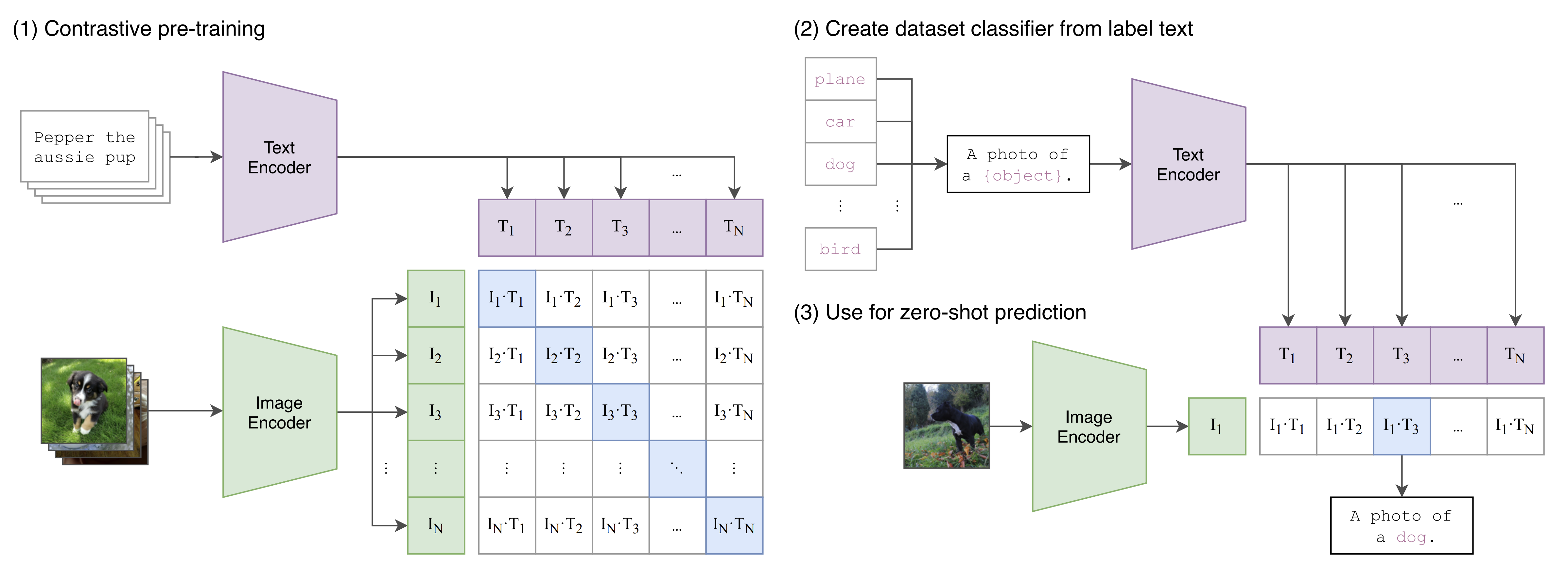 Fig 1. A summary of CLIP’s method [6].
Therefore, the optimization is based on a symmetric cross-entropy loss computed over these similarity scores, which is calculated by \(\frac{loss_i + loss_t}{2}\), where \(loss_i\) represents the loss of mapping description to image and \(loss_t\) is the loss of mapping image to description. The pseudocode for an implementation of CLIP from the original paper is shown below:
# image_encoder - ResNet or Vision Transformer
# text_encoder - CBOW or Text Transformer
# I[n, h, w, c] - minibatch of aligned images
# T[n, l] - minibatch of aligned texts
# W_i[d_i, d_e] - learned proj of image to embed
# W_t[d_t, d_e] - learned proj of text to embed
# t - learned temperature parameter

# extract feature representations of each modality
I_f = image_encoder(I) #[n, d_i]
T_f = text_encoder(T) #[n, d_t]

# joint multimodal embedding [n, d_e]
I_e = l2_normalize(np.dot(I_f, W_i), axis=1)
T_e = l2_normalize(np.dot(T_f, W_t), axis=1)

# scaled pairwise cosine similarities [n, n]
logits = np.dot(I_e, T_e.T) * np.exp(t)

# symmetric loss function
labels = np.arange(n)
loss_i = cross_entropy_loss(logits, labels, axis=0)
loss_t = cross_entropy_loss(logits, labels, axis=1)
loss = (loss_i + loss_t)/2
After training, the model is able to zero-shot transfer during inference. For example, CLIP combines can generalize to unseen object categories in image classification by predicting which text snippet should be paired with a given image, leveraging the names of all classes in a target dataset as potential text pairings. The process involves computing feature embeddings for both the image and the possible texts using their respective encoders. The cosine similarity of these embeddings is then scaled and normalized into a probability distribution via softmax, facilitated by a temperature parameter \(\tau\). Essentially, CLIP functions as a multinomial logistic regression classifier with L2-normalized inputs and weights, devoid of bias, and with temperature scaling. The image encoder acts as the computer vision backbone, generating a feature representation for the image, while the text encoder serves as a hypernetwork, generating weights for a linear classifier based on the text descriptions of the visual concepts represented by the classes. Once computed by the text encoder, the zero-shot classifier is cached and reused for subsequent predictions, optimizing computational cost across the dataset’s predictions. This process is illustrated in sections (2) and (3) of Figure 1.
CLIP: Zero-shot Evaluation
The performance of CLIP varies across different image classification datasets. To demonstrate its zero-shot capability, it is compared with a supervised Resnet-50 baseline. It demonstrates a slight advantage in general object classification datasets but shows particularly impressive results for the STL10 dataset, achieving a new SOTA result at the time. However, CLIP’s performance is weaker when it comes to specialized, complex, or abstract tasks such as satellite image classification, sign recognition, and lymph node tumor detection. These tasks require a higher degree of specificity and complexity that CLIP may struggle to handle effectively. Figure 2 shows the complete comparison.
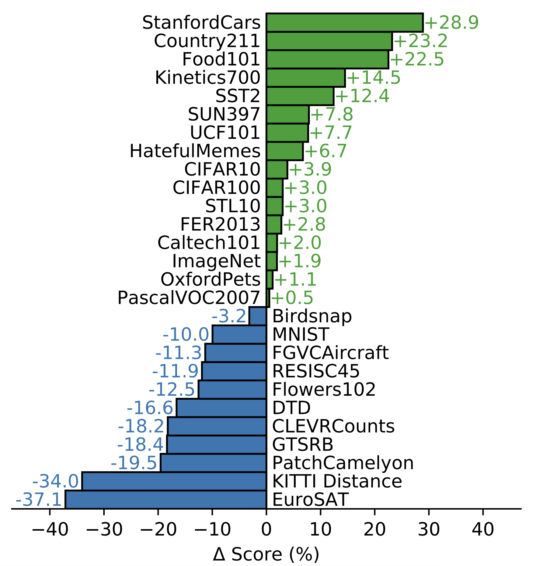 Fig 2. Zero-shot evaluation of clip against a supervised Resnet-50 baseline [6].
The Influence of CLIP
Although originally formulated for an image-classification task, many model adapt CLIP for a wide range of vision-related tasks. One such example is GLIP, which we will briefly introduce now.
GLIP: Extending CLIP for Grounding
GLIP (Grounded Language-Image Pre-training) [2] is a system that builds upon the capabilities of CLIP by incorporating object-level, language-aware, and semantic-rich visual representations. While CLIP made strides by learning directly from text-image pairs on the internet, GLIP extends this by learning not only from detection data but also from grounding data. This allows the model to not just recognize objects in images, but also to understand and ground the textual descriptions related to these images, enabling more precise and context-aware image understanding.
Introduced in the paper “Grounded Language-Image Pre-training” as an extension of the CLIP model, GLIP’s key advantage lies in its ability to conduct phrase grounding and object detection simultaneously. By unifying these two tasks, GLIP can provide precise, object-level visual representations with a semantic understanding that is language-aware. Compared to CLIP, whose understanding is at the image level, GLIP results in a richer and more detailed understanding of images. The model’s also allows for robust zero-shot learning capabilities. Additionally, the support for prompt tuning makes GLIP highly adaptable and efficient at learning new tasks. Figure 2 shows an overview of the framework of GLIP, which unifies detection and grounding.
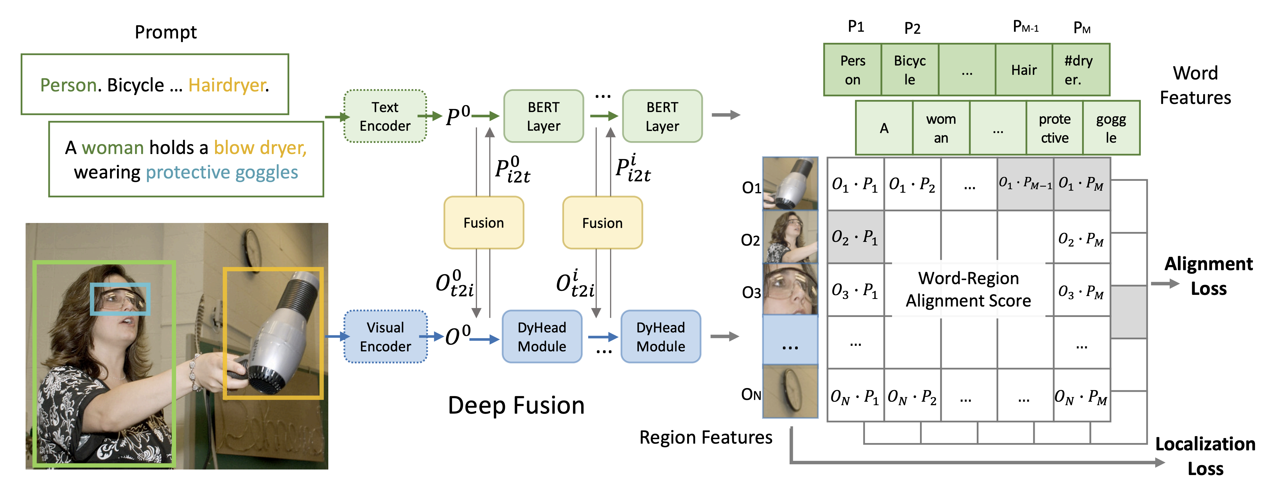 Fig 2. An overview of the framework of GLIP [2].
Using CLIP in Other Models: Sora
In addition to being adapted or extended, CLIP or CLIP-like modules are also widely used as a part of larger models. One of the large vision models that received a lot of attention recently is Sora, a text-to-video generative AI model released by OpenAI in February 2024. Sora is an example of using CLIP’s methods in larger vision models. A recent work [4], which reviews Sora, provides a reverse engineering of Sora’s framework. As a diffusion transformer, Sora uses latent diffusion to generate videos. This process is guided by the text from user input, achieved using a CLIP-like conditioning mechanism to guide the diffusion model to generate styled or themed videos. Figure 3 shows this reverse-engineered framework.
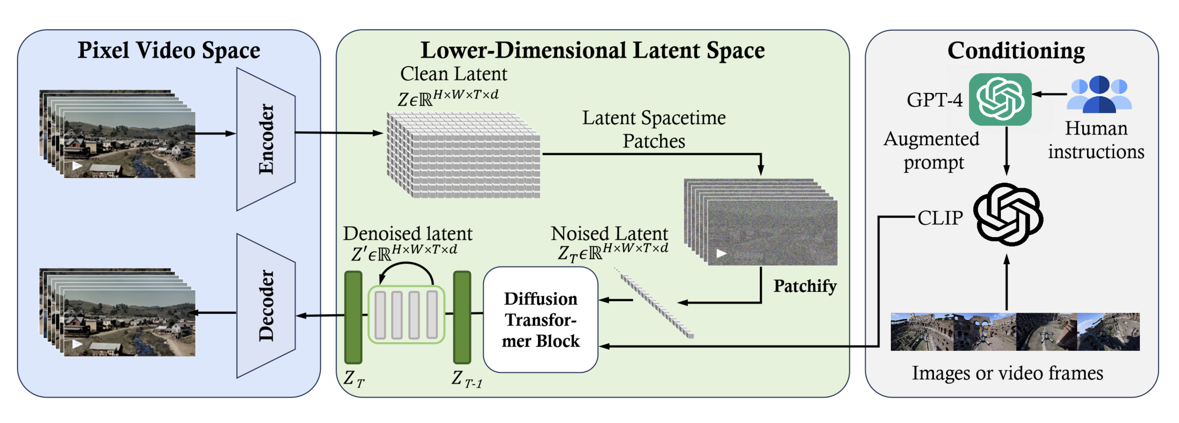 Fig 3. An overview of Sora’s framework, reverse-engineered. [4].
Shared Limitations: Fine-grained Understanding and Alignment
Experiment: Zero-shot Evaluation of CLIP against Supervised Baseline
As discussed previously when introducing CLIP, CLIP does have its limitations. One such issue is the performance on fine-grained, abstract, or out-of-distribution data. To verify this, we perform experiments to examine the zero-shot performance on the classic MNIST dataset. The intuition is that although it is a fairly simple task that has existed for a long time, such data might not be as abundant in common web collection, as usual images are not just a single digit with the corresponding natural language description like “the number 8.” We compare the CLIP with a pre-trained Resnet-50 model fine-tuned on MNIST by us.
After importing necessary libraries, we first prepare the dataset and fine-tune on a pre-trained Resnet-50:
transform = transforms.Compose([
    transforms.Resize(256),
    transforms.CenterCrop(224),
    transforms.Grayscale(num_output_channels=3),
    transforms.ToTensor(),
    transforms.Normalize(mean=[0.485, 0.456, 0.406], std=[0.229, 0.224, 0.225]),
])

train_dataset = datasets.MNIST(root='./data', train=True, download=True, transform=transform)
test_dataset = datasets.MNIST(root='./data', train=False, download=True, transform=transform)

train_loader = DataLoader(train_dataset, batch_size=64, shuffle=True)
test_loader = DataLoader(test_dataset, batch_size=64, shuffle=False)

# Modify ResNet50 for MNIST (10 classes)
resnet50 = models.resnet50(pretrained=True)
# Replace the final layer with a new layer that has 10 outputs
resnet50.fc = nn.Linear(resnet50.fc.in_features, 10)

# Move the model to GPU if available
device = torch.device("cuda" if torch.cuda.is_available() else "cpu")
print("Device:", device)
resnet50.to(device)

# Train the Model
criterion = nn.CrossEntropyLoss()
optimizer = optim.Adam(resnet50.parameters(), lr=0.001)

# Training loop
epochs = 5
for epoch in range(epochs):
    resnet50.train()
    running_loss = 0.0
    for images, labels in tqdm(train_loader, desc=f"Epoch {epoch+1}/{epochs}"):
        images, labels = images.to(device), labels.to(device)

        optimizer.zero_grad()
        outputs = resnet50(images)
        loss = criterion(outputs, labels)
        loss.backward()
        optimizer.step()

        running_loss += loss.item()
    print(f"Epoch {epoch+1}, Loss: {running_loss / len(train_loader)}")

# Evaluate
resnet50.eval()
correct = 0
total = 0
with torch.no_grad():
    for images, labels in tqdm(test_loader, desc="Evaluating"):
        images, labels = images.to(device), labels.to(device)
        outputs = resnet50(images)
        _, predicted = torch.max(outputs.data, 1)
        total += labels.size(0)
        correct += (predicted == labels).sum().item()

print(f'Accuracy of the network on the test images: {100 * correct / total:.2f}%')
As shown above, we replace the final layer and train the model for 5 epochs with lr=1e-3 using Adam optimizer. Then, we also evaluate on CLIP in a zero-shot fashion:
# # Load CLIP model and processor
clip_model = CLIPModel.from_pretrained("openai/clip-vit-base-patch32")
clip_processor = CLIPProcessor.from_pretrained("openai/clip-vit-base-patch32")

# Define MNIST labels as text prompts for CLIP
label_prompts = [f'a photo of the number: "{i}".' for i in range(10)]

# MNIST dataset preprocessing: Convert to RGB and Resize to match CLIP's input size
mnist_transform = transforms.Compose([
    transforms.Resize((224, 224)), # Resize to match CLIP's input dimensions
    transforms.Grayscale(num_output_channels=3), # Convert to 3-channel grayscale
    transforms.ToTensor(),
])

# Load MNIST test dataset
mnist_test = MNIST(root='./data', train=False, download=True, transform=mnist_transform)
test_loader = DataLoader(mnist_test, batch_size=32, shuffle=False)

def predict_clip_zero_shot(model, processor, images, text_prompts):
    # Process the images and texts
    inputs = processor(text=text_prompts, images=images, return_tensors="pt", padding=True)

    # Get the logits from the model
    with torch.no_grad():
        outputs = model(**inputs)
        logits_per_image = outputs.logits_per_image # shape: (num_images, num_texts)
        probs = logits_per_image.softmax(dim=1) # Softmax over the texts dimension

    # Predict the most likely text for each image
    return probs.argmax(dim=1)

total_correct = 0
total_images = 0

for images, labels in tqdm(test_loader, desc="Evaluating", leave=True):
    images_pil = [transforms.ToPILImage()(image) for image in images]
    predictions = predict_clip_zero_shot(clip_model, clip_processor, images_pil, label_prompts)
    total_correct += (predictions == labels).sum().item()
    total_images += labels.size(0)

accuracy = total_correct / total_images
print(f"CLIP Zero-Shot Accuracy on MNIST: {accuracy * 100:.2f}%")
The resulting performance difference is drastic: Our simple fine-tuned Resnet baseline achieves a test accuracy of 99.18% in 5 epochs, whereas the zero-shot CLIP only has 52.50%. This difference is greater than the reported result in the original CLIP paper, and upon investigating, many people experienced similar issues. Regardless, it demonstrates how CLIP can have very mediocre performance on even simple datasets.
As a comparison, we also evaluate on the CIFAR10 dataset. Due to the similarity with common web data, we expect a closer performance.
clip_model = CLIPModel.from_pretrained("openai/clip-vit-base-patch32")
clip_processor = CLIPProcessor.from_pretrained("openai/clip-vit-base-patch32")

cifar_transform = transforms.Compose([
    transforms.Resize((224, 224)),  # Resize to match CLIP's input dimensions
    transforms.ToTensor(),
])

testset = datasets.CIFAR10(root='./data', train=False, download=True, transform=cifar_transform)
testloader = DataLoader(testset, batch_size=32)

classes = [
    'airplane',
    'automobile',
    'bird',
    'cat',
    'deer',
    'dog',
    'frog',
    'horse',
    'ship',
    'truck',
]

prompts = [f'a photo of a {i}.' for i in classes]

def predict_clip_zero_shot(model, processor, images, text_prompts):
    inputs = processor(text=text_prompts, images=images, return_tensors="pt", padding=True)

    with torch.no_grad():
        outputs = model(**inputs)
        logits_per_image = outputs.logits_per_image # shape: (num_images, num_texts)
        probs = logits_per_image.softmax(dim=1) # Softmax over the texts dimension

    return probs.argmax(dim=1)


total_correct = 0
total_images = 0

for images, labels in tqdm(testloader, desc="Evaluating", leave=True):
    images_pil = [transforms.ToPILImage()(image) for image in images]
    predictions = predict_clip_zero_shot(clip_model, clip_processor, images_pil, prompts)
    total_correct += (predictions == labels).sum().item()
    total_images += labels.size(0)

accuracy = total_correct / total_images
print(f"CLIP Zero-Shot Accuracy on MNIST: {accuracy * 100:.2f}%")
The evaluation on CIFAR-10 using CLIP gives a test accuracy of 85.16%. Our Resnet-50 result is 89.22%, which confirms our hypothesis.
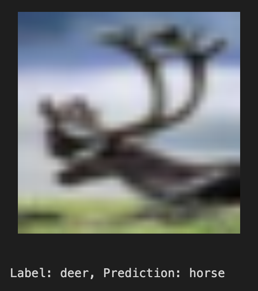
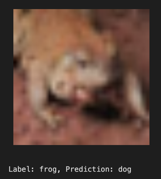
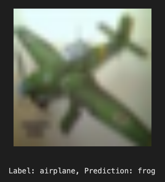
Here are some examples where CLIP fails:
| Deer | Frog | Airplane |
|---|---|---|
 |
 |
 |
Beyond CLIP: Challenges with Fine-Grained Alignment
The issue of CLIP is not unique to itself but also with models derived from it and large vision-language models in general. For example, one work, DesCo [3], that build on the GLIP model we introduced pointed out issues in models like GLIP when the input contains rich language descriptions. They found that the models often ignore the contextual information in language descriptions and takes shortcuts by only recognizing certain keywords without considering their semantic relationships. Models also hallucinate by identifying objects that don’t exist. They pointed out the multi-fold nature of the problem. The relatively obvious yet still hard to resolve cause is the lack of fine-grained descriptions in image-caption data that used in training current vision-language models. This resembles the reporting bias phenomenon: when writing captions for images, humans tend to directly mention the entities rather than give a detailed description. The more challenging issue is that even provided with data rich in descriptions, models often lack the incentive to leverage these descriptions effectively. This requires careful setup of the contrastive training goal and robust design of negative samples. Figure 4 shows an overview of their work by comparing prior methods which struggle in said scenarios vs. their improvements.
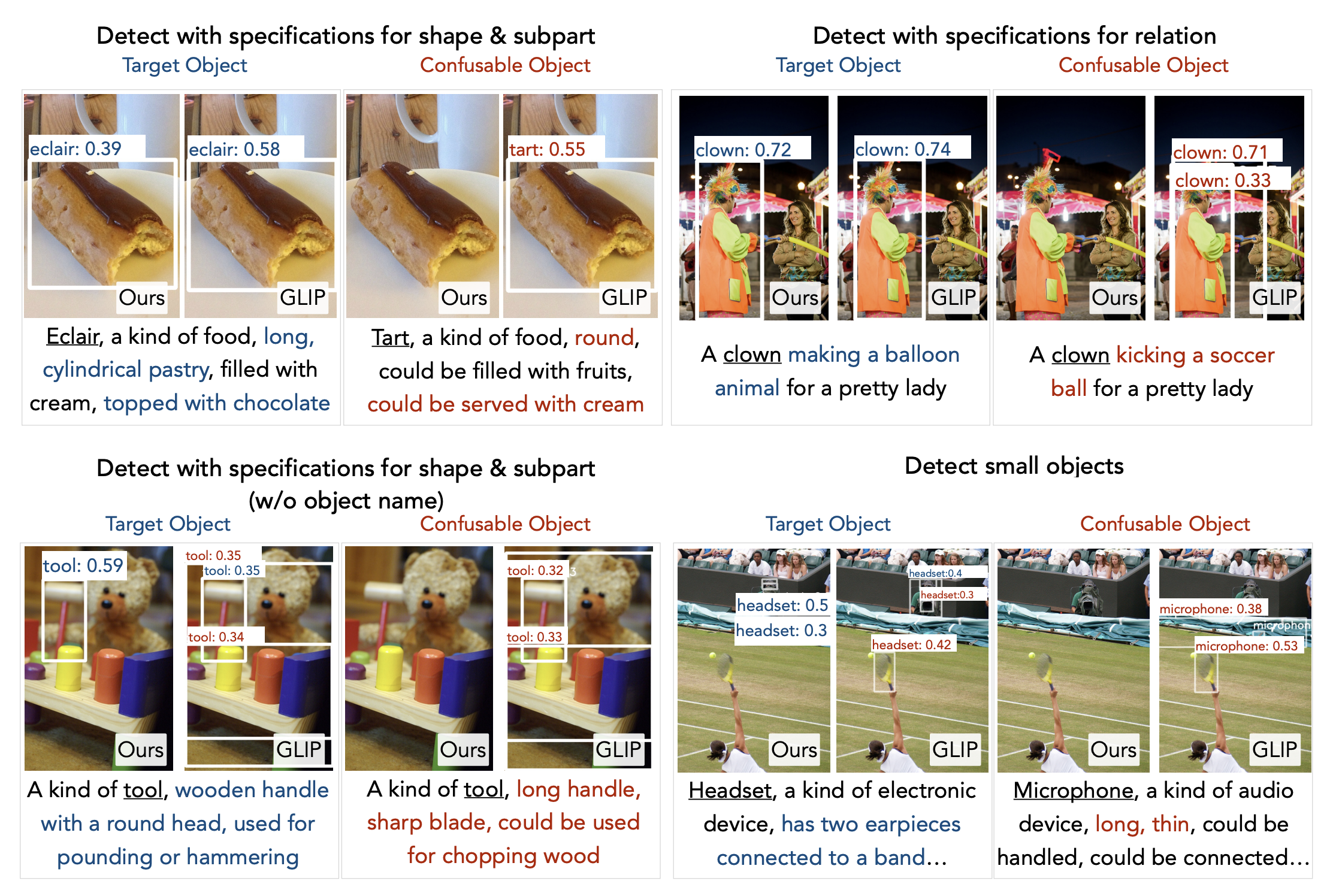 Fig 4. An overview of the DesCo [3].
Even in larger models, we can see traces of such issues. A recent benchmark ConTextual [8] reveals the significant limitations that current large multimodel models have in terms of text-rich visual reasoning in complex tasks involving joint reasoning over text and visual content in the image (e.g., navigating maps in public places). Even the best-performing LMM on the benchmark, GPT-4V, has a significant performance gap of 30.8% compared with the human counterpart. For example, some LMMs often cannot correctly identify the time from a picture of the clock and often produces a fixed result. They also struggle on abstract tasks requiring systematic steps and back-and-forth reasoning between the image and the text prompts. Figure 5 shows some examples.
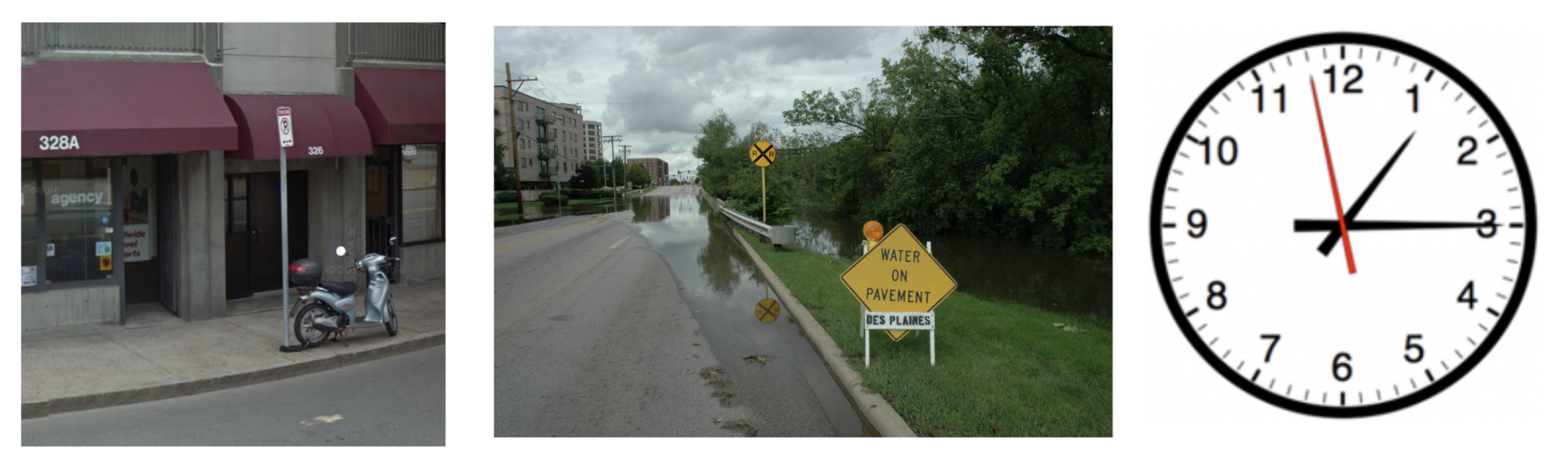 Fig 5. Examples from the ConTextual benchmark [8].
The issues identified can be summarized into two core aspects: (1) getting data with rich, fine-grained details and (2) leveraging such data by formulating a better contrastive pre-training setup. DesCo [3] attempted to resolve the problem in both directions. Specifically, it aims to leverage rich description on the text side by generating detailed text information. Similarly, it would be interesting to explore leveraging image generation models to enrich the training data on the image side for better vision-language alignment. For example, controlled manipulation through models like ControlNet [8] and FreeControl [5] can be potentially useful in constructing contrastive samples for better vision-language alignment.
Conclusion
We started from introducing CLIP, its methods, and influences in the advancements in large vision-language models. We surveyed different works that builds on or uses CLIP and how they contribute to the trend of ultra large-scale models in today’s computer vision. We then identified limitations of CLIP, and extended to similar weaknesses in large vision-language models in general. We identified a common issue in some of there shared limitations, namely fine-grain vision-language alignment. To better understand this issue, we used some works to illustrate possible causes of the issue and discuss potential solutions towards better alignment in vision-language models.
References
[1] Chen, Radford, et. al. “Generative Pretraining From Pixels.” Proceedings of the 37th International Conference on Machine Learning, PMLR 119:1691-1703, 2020.
[2] Li, Zhang, et. al. “Grounded Language-Image Pre-training.” CVPR, 2022.
[3] Li, Dou, et. al. “DesCo: Learning Object Recognition with Rich Language Descriptions.” NeurlIPS, 2023.
[4] Liu, Zhang, et. al. “Sora: A Review on Background, Technology, Limitations, and Opportunities of Large Vision Models.” arXiv:2402.17177v2 [cs.CV].
[5] Mo, Mu, et al. “FreeControl: Training-Free Spatial Control of Any Text-to-Image Diffusion Model with Any Condition” CVPR, 2024.
[6] Radford, Kim, et al. “Learning Transferable Visual Models From Natural Language Supervision.” International Conference on Machine Learning, 2021.
[7] Tian, Krishnan, et. al. “Contrastive Multiview Coding.” arXiv:1906.05849v5 [cs.CV].
[8] Wadhawan, Bansal, et al. “CONTEXTUAL: Evaluating Context-Sensitive Text-Rich Visual Reasoning in Large Multimodal Models.” arXiv:2401.13311(2024).
[9] Zhang, Rao, et. al. “Adding Conditional Control to Text-to-Image Diffusion Models.” International Conference on Computer Vision, 2023.