Image Generation
In this project I will provide a brief overview of the history of generative modeling with respect to computer vision and dive into an application of the transformer architecture to the field.
- Image Generation: A Brief History
- What is Diffusion?
- Old Architectures for diffusion
- DiT
- My Results
- Future Work and Improvements
- Reference
Image Generation: A Brief History
With the growth of generative modeling in the last three years, in part spurred by the rapid adoption of ChatGPT, I decided to explore image generation. Let’s get out bearings by briefly covering some of the history of generative modeling, and its relations to image generation.
Classical Approaches to Generative Modeling
In the past, there have been two classes of generative modeling: implicit and likelihood based.
- Implicit models attempt to model the sampling process of the data distribution rather than the data distribution itself. The main architecture that emerged from this approach is Generative Adversarial Networks (GANs)
- Likelihood based models attempt to learn the actual probability distribution of the data using some form of maximum likelihood Estimation. Many architectures emerged from this approach, including Autoregressive Models (ARMs), Variational Autoencoders (VAEs), and Vector-Quantized VAEs (VQ-VAEs) These two approaches have some major issues that affect the capabilities of any architectures that emerge from these fields. GANs for example, require unstable adversarial training, which could lead to mode collapse. Likelihood based models, on the other hand, face issues when calculating the normalizing constant of the probability distributions that they are modeling. In short these models parameterize the probability distribution as \(p_\theta(x)=\frac{e^{-f_{\theta}(x)}}{ Z_{\theta}}\) where \(Z_\theta\) is the normalizing constant. Calculating that constant can become intractable, which limits the model’s effectiveness and the complexity that it can attain. This is where score based modeling can help
The New Approach: Score Based Generative Modeling
There are three critical components to score based generative modeling:
- The score function: \(s_{\theta}(x) = \nabla_{x}\log p_\theta(x)\)
- Score Matching: A family of algorithms that can minimize the fisher divergence between two distributions without actually calculating the score function of our data distribution
- Langevin Dynamics: An iterative sampling process that uses the score from to generate new samples from its distribution. Each of these subjects deserves its own deep dive, but for times sake, I’m going to quickly show you how this solves the issue of intractable constants within likelihood based modeling: \(s_{\theta}(x) = \nabla_{x}\log p_\theta(x) = \nabla_{x}\log\frac{e^{-f_{\theta}(x)}}{ Z_{\theta}} = -\nabla_{x}f_{\theta}(x) - \nabla_{x}\log Z_{\theta} = -\nabla_{x}f_{\theta}(x)\) As you can see we’ve eliminated the normalization constant through some log manipulation and gradients. This makes our lives easier, and removes that constraint on our models and their architecture.
What is Diffusion?
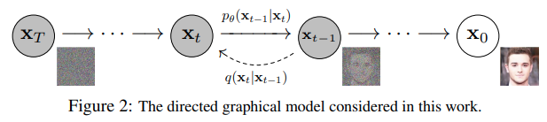 Fig 1. An Illustration of the Diffusion Process [1].
Diffusion is the process that we will use to generate a new image. It can be decomposed into three broad steps:
- Take an example, add noise according to a noise schedule
- Train a model to predict the noise that was added at any given timestep
- Iteratively denoise pure noise until you’ve arrived at a useful image
Math
Let’s define this approach more mathematically: given that \(q_0(x)\) is a data distribution, we will define the forward process as \(q(x_t\|x_{t-1})\) given some covariance schedule \(0<B_1<\cdots<B_T<1\) where \(q(x_t\|x_{t-1})= N(x_t, \sqrt(1-B_t)x_{t-1}, B_t)\) This adds noise of increasing variances to the examples as we progress through time. Through a few tricks we can arrive at a much simpler formulation that we discussed in assignment 4, namely that by creating \(\alpha_t = 1-B_t\) and \(\bar{\alpha}_t = \Pi_{i=0}^t\alpha_i\) we can reparameterize the above equation as \(x_t = \sqrt{\bar{\alpha}_t}x_0+\sqrt{1-\bar{\alpha}_t}\epsilon\) where epsilon is noise sampled from a unit normal distribution.
Why add Noise?
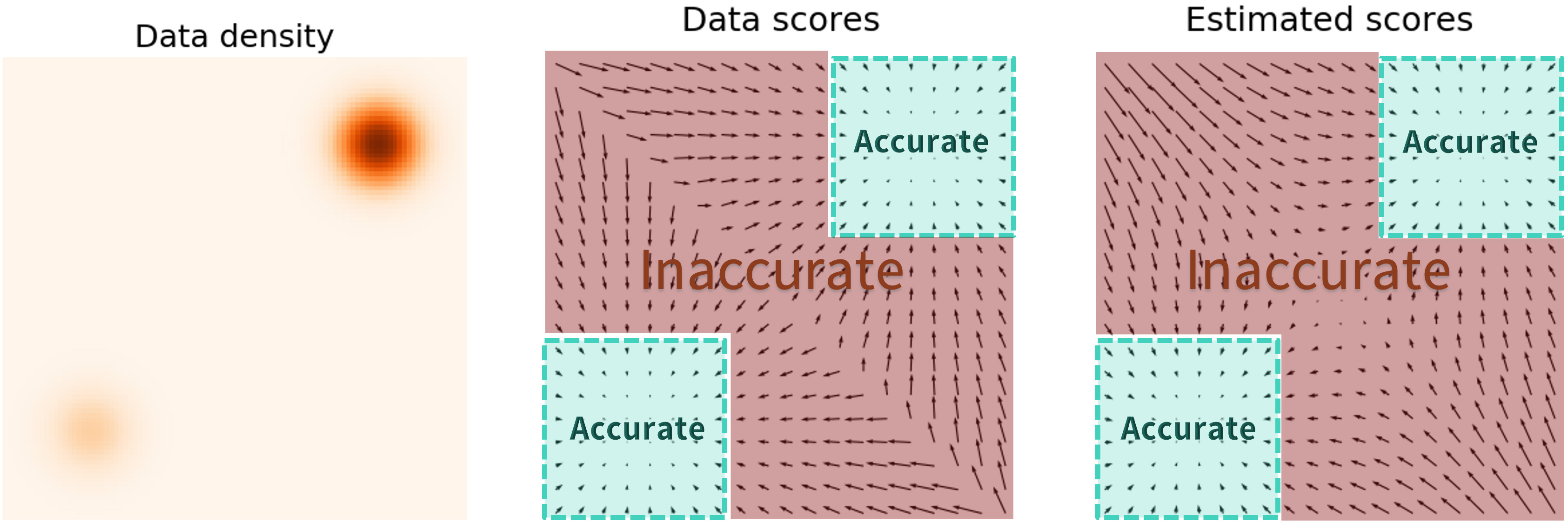 Fig 2. Estimated scores in a probability distribution with no perturbation [2].
When we don’t perturb the data distribution, there exist regions of high probability density, and regions where there is practically none. In this case, there is a clear issue in that if we start at some random position far away from the areas of high density, its relatively unlikely for the score function to guide us back to a usable image.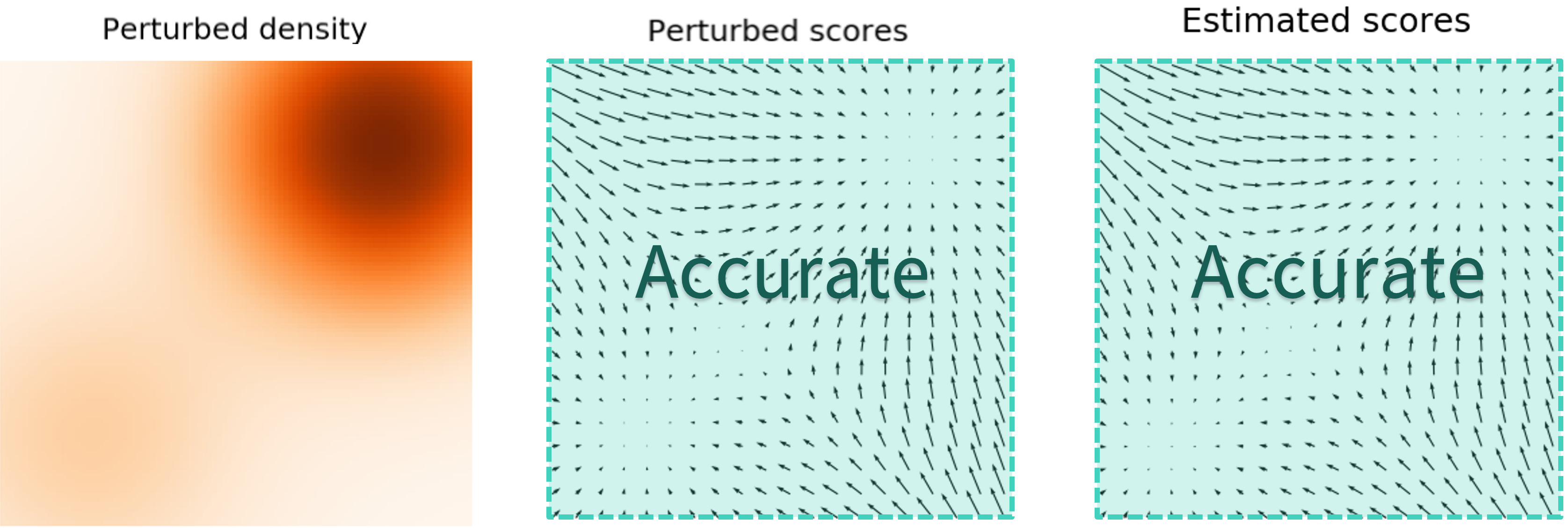 Fig 3. Estimated scores in a probability distribution with perturbation [2].\
When we perturb the distribution with noise, we artificial shift the probability density to be more uniform. Therefore by adding noise we create a more accurate score function, and thus more reliable sampling.
Old Architectures for diffusion
There have been three major architectures for diffusion models in the past, each improving on the past. The first was the DDPM denoising diffusion probabilistic model or DDPM. This was the original diffusion model introduced in 2020 by Ho et al.[3] This is the formulation that I have presented above, adding noise, and then using a U-Net architecture to predict noise and sample back to an image. DDPM was followed shortly by denoising diffusion probabilistic models or DDIM introduced by Song et al.[4] DDIM used exactly the same training goal and forward process as DDPM but made improvements to sampling by redefining the process as a non-markovian one. This led to major speed ups over the original DDPM Finally there is the latent diffusion models or LDM. Rather than making changes to the formulations of the problem, LDM exploits the latent space of a pretrained VAE.[5] Operating in the latent space has its advantages, as operating in the lower dimensional space improves model performance for minimal tradeoff in quality.
The U-Net
All of these approaches, until recently, have used a U-Net architecture to predict the noise that was added to images. Originally used for medical image segmentation[6], the U-Net aggressively downsamples an input image in order to extract only the most important features. Once that is complete, it upsamples from those rich features back to the original image dimensions. The only major modification that has to be made to this network for diffusion can be seen in the figure below, that being a timestep embedding being included in each block.
 Fig 4. Adapted U-Net Architecture for Diffusion [7].\
Attention vs Convolutions
The U-Net architecture utilizes convolutions throughout its process, as it was the standard approach to image processing operations. It has many advantages, including the ability to capture spatial information from input, and the sparsity of the weights.
However, with the dawn of the attention mechanism, its become clear that convolutions are less effective in information capture across sequences. The key reason is the concept of receptive fields. With a convolution, our receptive field, or more informally, the inputs that effect our output, is only the size of the filter that we use. With the attention mechanism, our receptive field is effectively the whole input sequence of patches. In effect, when using attention we will “see” the entire image at each layer, rather than only a small part of it.
DiT
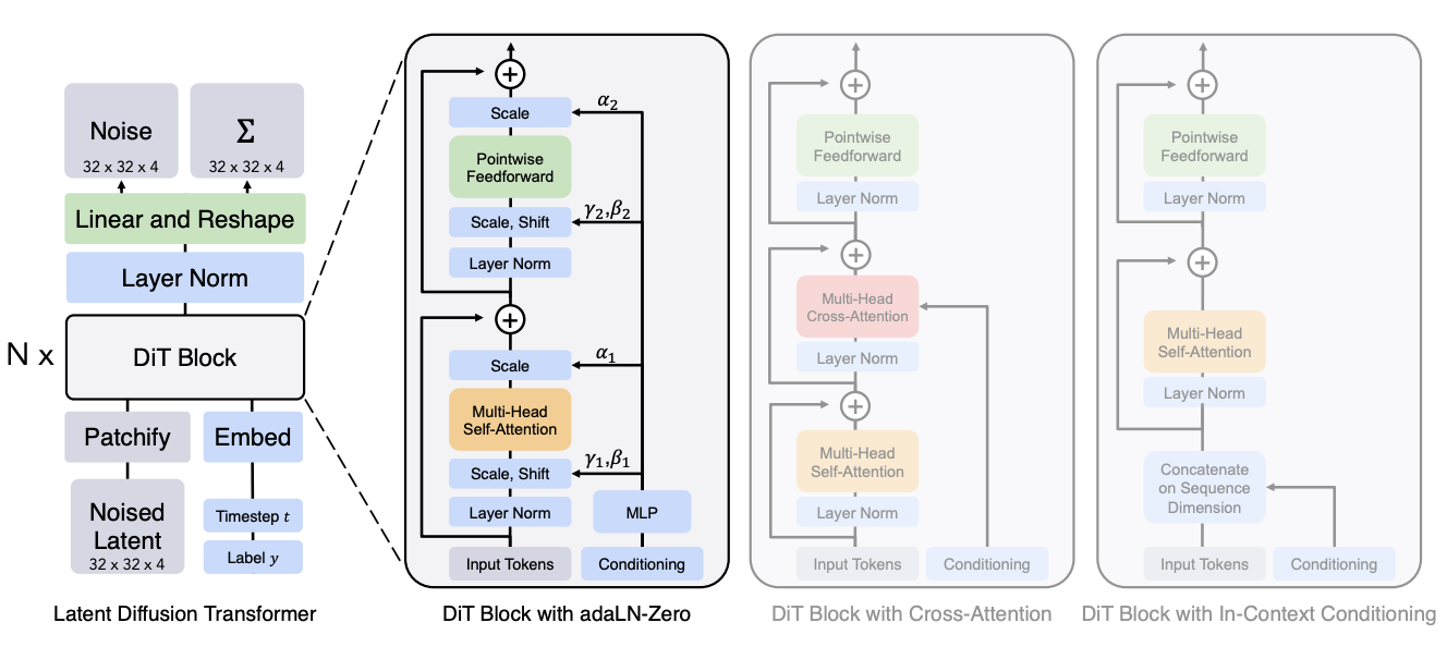 Fig 5 DiT Architecture with Differing Conditioning Approaches [8].
That leads us to Diffusion Transformers. Like other transformers, it first converts the input into a series of patches using a convolutional embedder, and then passes the input through a multiheaded attention module. The paper introduced 4 different mechanisms for conditioning on timestep and label of image for classifier free guidance.
- In Context Conditioning: attach the embedded condition to the input, similar to a cls token in segmentation.
- Cross Attention: apply cross attention between the embedded conditions after the multihead attention block.
- Adaptive Layer Norm (AdaLN): an adaptive layer normalization technique, where you regress the parameters from the embedding vectors.
- Adaptive Layer Norm-Zero (AdaLN-Zero): same method as before, but with initializing of the transformer blocks as the identity function. \
AdaLN and AdaLN-Zero both added negligible flops to the model, while maintaining good performance, whereas in context adds slightly more, and cross attention adds “roughly a 15% overhead” to the model in terms of flops. In practice the diffusion transformer performed very well relative to other U-Net based models, as can be seen below:
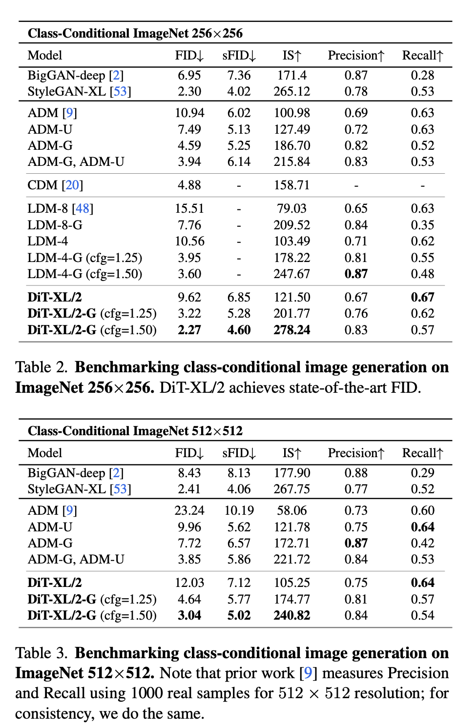 Fig 5 DiT Results [8].
In this table ADM is a traditional U-Net diffusion model without the use of a latent space. LDM is a latent diffusion model using a U-Net, and the DiT tested was a latent diffusion architecture. It performs better than both models on FID and sFID. Additionally in the paper it is specified that ADM uses an order of magnitude more operations than LDM and DiT, with LDM and DiT having a similar number of operations.
This result is important because it demonstrates the feasibility of using transformers in a diffusion setting. With the growth of diffusion as a tool not only for image generation, but scene generation and beyond, this means that we can utilize the more efficient and effective transformer architecture wherever we are intending on using diffusion.
My Results
I decided that I’d give DiT a try, and set out with the main goal of comparing the limits of the architecture in low data environments. To accomplish this I decided to train a U-Net and DiT on the fashionmnist datasets and see how they compared.
During this work I attempted to make the models comparable in size and training time, but due to time constraints I was unable to verify their relative complexity other than by wall clock time. The DiT, with three layers, an expansion factor of 384 and six attention heads trained slower, by nearly ten minutes in some runs, than a small U-Net model. This verifies that transformers in general will be slower than CNNs to train. As we can see below, the quality of the images generated between the two architectures is comparable after the same number of training iterations.
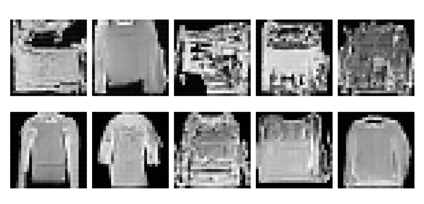 Fig 5 DiT Generated Images [8].
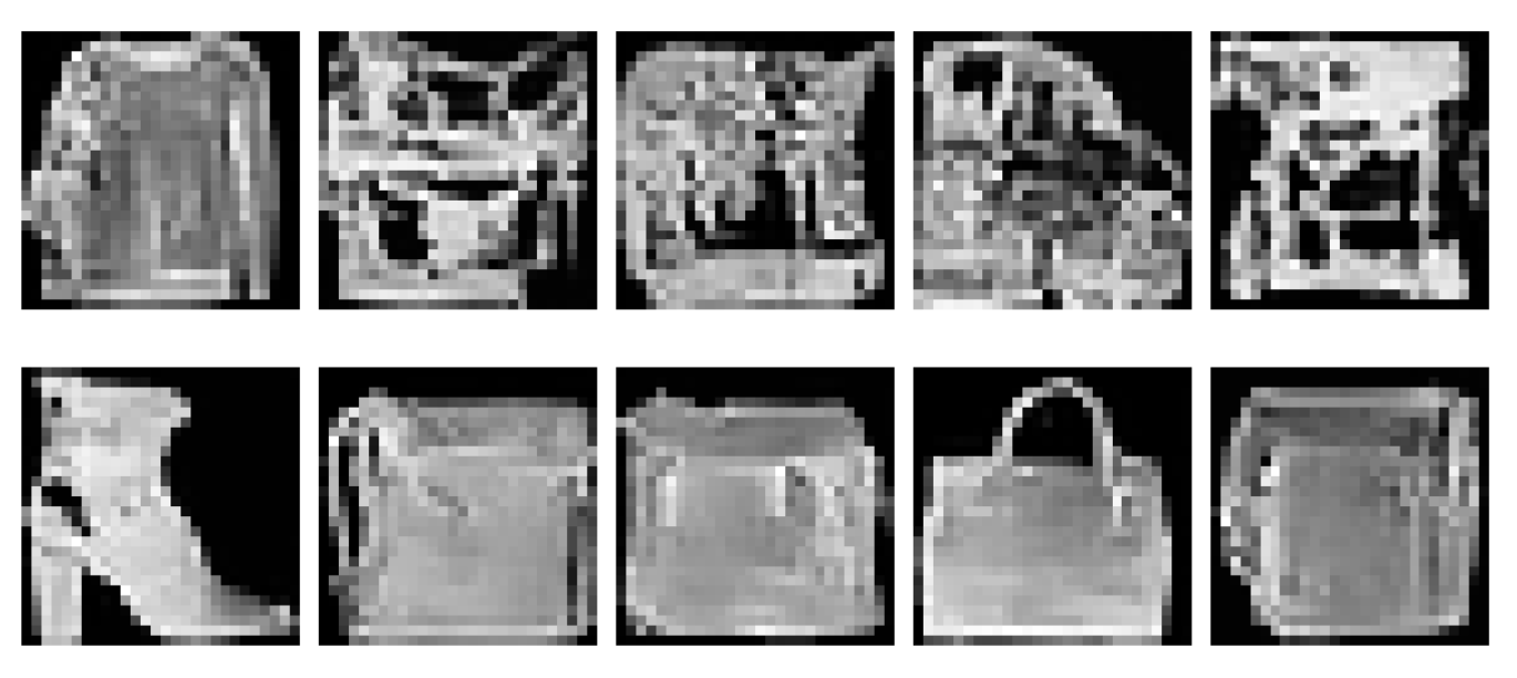 Fig 5 U-Net Generated Images [8].\
Future Work and Improvements
In the future I would like to explore the use of classifier free guidance in training diffusion models, perhaps implementing that with a simple U-Net before moving to a transformer architecture, as I didn’t have time to work on that over the course of this quarter. Further I would like to extend into using the CIFAR-10 Dataset to get more clear results between the two model backbones. Additionally within my work, I chose to avoid working with a latent diffusion approach to generating images for simplicity’s sake. The next step to improving the training and sampling time of my models would be to implement a latent diffusion approach. Finally, there has been quite the stir about a newer architecture, Mamba, or selective state space models[10], which appear to have some promise as a newer architecture. It would be interesting to explore how they perform relative to transformer based architectures.
Reference
My code can be found at here
[1] “The Annotated Diffusion Model.” Hugging Face – The AI Community Building the Future., huggingface.co/blog/annotated-diffusion/, 2022
[2] Song, Yang. “Generative Modeling by Estimating Gradients of the Data Distribution”
https://yang-song.net/blog/2021/score/, 2021
[3] Ho et al. “Denoising Diffusion Probabilistic Models” 34th Conference on Neural Information Processing Systems, 2020.
[4] Song et al. “Denoising Diffusion Implicit Models” International Conference on Learning Representations, 2021.
[5] Rombach et al. “High-Resolution Image Synthesis with Latent Diffusion Models” Conference on Computer Vision and Pattern Recognition, 2022.
[6] Ronneberger et al. “U-Net: Convolutional Networks for Biomedical Image Segmentation” International Conference on Medical Image Computing and Computer-Assisted Intervention, 2015.
[7] D., Prince Simon J. “Understanding Deep Learning.” The MIT Press, 2023.
[8] Peebles et al. “Scalable Diffusion Models with Transformers” International Conference on Computer Vision, 2023.
[9] Gu et al. “Mamba: Linear-Time Sequence Modeling with Selective State Spaces”, 2023.