Object Tracking
Object tracking has been a prevalent Computer Vision task for many years with many different deep learning approaches. In this report, we will explore the inner workings of two different approaches, DeepSORT for multiple object tracking and SiamRPN++ for single object tracking, comparing and contrasting their capabilities. We also briefly look at ODTrack, a more recent tracking algorithm. Finally, we have a short demo on DeepSORT with YOLOv8.
Introduction
Object Tracking is a CV task that automatically detects objects as they move through a video frame by frame. Typically, a video is fed into an object tracking algorithm and the algorithm outputs a set of coordinates creating a box that surrounds the object(s) being tracked in each frame. These boxes are called bounding boxes. An example video can be seen below.
Object tracking is applicable to many different tasks. Autonomous vehicles need to use object tracking to detect pedestrians, other cars, and obstacles that it needs to avoid and monitor. Implementing automatic video surveillance can identify people and other objects of interest without the need for human intervention. It has the ability to streamline tasks and revolutionize many industries.
In this report, we will explore different deep learning algorithms and approaches to object tracking that have been used throughout the years.
Challenges
There are a few main challenges that researchers have been tackling within the object tracking paradigm. They all have to do with noise in the sensory data, mainly the camera footage. The most common issue is occlusions where objects being tracked are partially blocked by other objects or the background. This leads to a change of appearance that makes it hard to identify the object in subsequent frames, leading to inaccuracy in tracking. As a result, many algorithms have been developed to combat this problem. Other cases of noise include when the camera has low illumination of camera footage, non-rigid transformation of target objects where the state of the object changes dramatically, camera movement, hard to track features, background clutter, and boundary effects. Additionally, as with many applications, performance and efficiency are important.
Aproaches
SiamRPN++
First, we will dive into single object tracking which is applicable when you want to track a specific target within a video. A popular framework used throughout the years is SiamRPN which utilizes a Siamese Network as a backbone feature extractor and then region proposal networks to predict the bounding box of the target object with video frames [2].
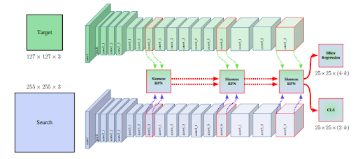
Fig 1. SiamRPN++ architecture with ResNet50 backbone, layer wise aggreagation, and RPN fusion for classification and bounding box regression [1].
Siamese Network
A Siamese Network consists of two identical networks that encode separate images into the same feature space to be used in a contrastive task. The idea is that since the networks are identical they can distinguish features of images that make them similar for a certain task. Similar images are embedded closer to each other while contrasting images have more different embeddings. SiamRPN utilizes a siamese network to compare what they call the target and search patches. The target patch of size \(127 \times 127 \times 3\) is often taken from the first frame of the video and contains the target object to be tracked. The search patches are \(255 \times 255 \times 3\) frames of the video where we want to track the object. We feed into the network one search frame at a time to identify where the target object is. Optimally, the siamese network encodes the patches into a space where search patches with target object features are closer to the target patch in the embedding space [1].
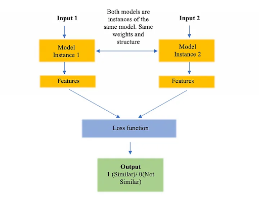
Fig 2. Diagram of a simple Siamese Network used for contrastive tasks. [1].
The backbone networks of the Siamese network in SiamRPN were originally AlexNets [1]. The utilization of a deep CNN architecture allowed for more robust feature representations of the target object despite occlusions, background clutter, and other obstacles to tracking. Additionally, it can represent objects that are harder to detect due to its improved ability to detect higher dimensional features.
Region Proposal Network (RPN)
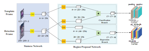
Fig 3. A representation of how the Siamese Network and RPN interact. [1].
The two patches or frames (now size \(6 \times 6 \times 256\) and \(22 \times 22 \times 256\)) are then thrown into a region proposal network. Region proposal networks, originally introduced as part of Faster-RCNNs, are used for object detection tasks to predict the bounding box coordinates and classify the object in the box. In the SiamRPN, they are used similarly where the regression branch predicts the anchor box transformation to get the bounding box of the target object in the search frame while the classification branch classifies whether each predicted box is background or the target object [1].
A critical differing component of the SiamRPN region proposal network is the cross correlation operation. Here, a convolution takes in the feature extraction from the detection (search) and template (target) branches and uses a convolutional layer to compute the correlation between them in order to predict where the target object is in the detection frame. The output of the regression branch is \(17 \times 17 \times 4k\) where k is the number of anchors. Bounding box coordinate outputs come in the form \((d x_l^{r e g}, d y_l^{r e g}, d w_l, d h_l)\) which can be used to transform the anchor box into the predicted bounding box for the target object. The transformation of the regression output to the predicted bounding box coordinates is given by the equation:
\[\begin{aligned} x_i^{p r o} & =x_i^{a n}+d x_l^{r e g} * w_l^{a n} \\ y_j^{p r o} & =y_j^{a n}+d y_l^{r e g} * h_l^{a n} \\ w_l^{p r o} & =w_l^{a n} * e^{d w_l} \\ h_l^{p r o} & =h_l^{a n} * e^{d h_l} \end{aligned}\]where the anchor box coordinates are given as \((x_i^{a n}, y_j^{a n}, w_l^{a n}, h_l^{a n})\) [1]. The output of the classification branch is \(17 \times 17 \times 2k\) where for each anchor box we predict whether the box encapsulates the target object or background.
Loss function
\[\operatorname{smooth}_{L_1}(x, \sigma)= \begin{cases}0.5 \sigma^2 x^2, & |x|<\frac{1}{\sigma^2} \\ |x|-\frac{1}{2 \sigma^2}, & |x| \geq \frac{1}{\sigma^2}\end{cases}\]The loss function used in the SiamRPN is a weighted sum of smooth L1 loss for the regression branch and cross-entropy loss for the classification branch. Smooth L1 loss is a combination of L1 and L2 loss incorporating advantages for both. L1 loss is more robust to outliers so whenever the input is above a certain threshold \(1/\sigma^2\) we use it for easier optimization and to prevent exploding gradients. L2 loss is more smooth and differentiable so we use it when it is below \(1/\sigma^2\) for better optimization. Cross entropy is used due to the binary classification problem. The weighted sum loss allows us to flow gradients from the output all the way throughout the network in one backward pass. This is another positive of using a Deep Network since it allows for end to end optimization, streamlining the training process [1].
One Shot Detector
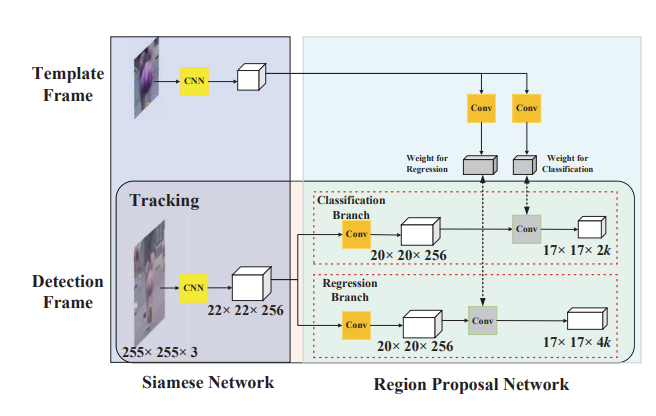
Fig 4. The template branch predicts the weights of the kernel (in gray) based on the first frame which is fused into the region proposal network as a convolutional layer. [1].
SiamRPN can also be shaped to become a one shot detector. It needs only one frame of the target object to be fed into the feature extractor for a single forward pass. Convolutional weights for the template branch are then determined through the gradients and incorporated into the detection branch as a cross correlation convolutional layer. These weights can be updated in further end to end optimization when detection frames are passed through the network. Since we no longer need the target frame, the template branch is removed from the network leading to a local detection network that is fed search frames from the video. This allows for more efficient optimization and inference [1].
For one shot detection, we need to adapt the proposal phase where we attempt to find the final bounding box for the object we are tracking. As a result, we need to eliminate some bounding boxes and only leave the best ones behind. SiamRPN uses a two step approach to rank boxes. First they only keep a \(g \times g\) subregion of proposed boxes that are near the center of the feature map of the detection frame. Anchors too far away are considered outliers. Then they use a cosine window to punish large displacement and scale change penalty to suppress large change to size and ratio. The mathematical formula used to rank the boxes is:
\[\text { penalty }=e^{k * \max \left(\frac{r}{r^{\prime}}, \frac{r^{\prime}}{r}\right) * \max \left(\frac{s}{s^{\prime}}, \frac{s^{\prime}}{s}\right)}\]where k is a hyperparameter, r is the ratio of height and width, and s is the overall scale of the proposal. In the end, the top K proposals generated from this equation are chosen then multiplied by the classification score to be evaluated using non max suppression. A final bounding box will be selected and linearly interpolated to image size [1].
SiamRPN++ Improvements
SiamRPN alone performs decently but there is an accuracy gap between it and algorithms that use deeper networks like ResNet50 to extract features. As mentioned above, SiamRPN utilizes AlexNet as its feature extraction backbone. Deeper networks have better capabilities to track higher dimensional features and perform much better on feature extraction as exemplified by improved performance on ImageNet. The authors of SiamRPN++ decided to use the SiamRPN architecture but to use ResNet50 as the feature extraction backbone instead of AlexNet because of these broad capabilities [2]. However, they needed to make a few adjustments in order to fully leverage the capabilities of the ResNet50 backbone.
Spatial Aware Sampling

Fig 5. Red indicates regions where positive samples are identified the most whereas blue is the opposite. As a result, higher shift increases the region of positive samples, increasing the area where target objects can be identified within the search frame. [2].
They noticed that once they added ResNet50 as the backbone, the model developed a strong center bias where they could only identify targets within the center of the search frame. This was due to the padding within ResNet50 that wasn’t present in AlexNet. As a result, they decided to use a spatial aware sampling algorithm to train the model. Basically, the idea was to set a hyperparameter called shift which would define the bounds of pixels that training images would be translated horizontally and vertically. How much they shifted within the bounds was random [2].
Depthwise Cross Correlation
Unlike the up-channel cross correlation, depth-wise performs the convolution operation independently between all the channels of the input. This causes no interactions within the different channels during the cross correlation operation. This is good for reducing the feature size efficiently with less parameters. Later on, another convolution would fuse the channels and determine the correlation. Additionally, with the up-channel cross correlation there was a great imbalance of parameters between the RPN and the feature extraction backbone that caused optimization to be unstable. With the depth-wise cross correlation layer, the number of parameters reduces greatly leading to better optimization [2].
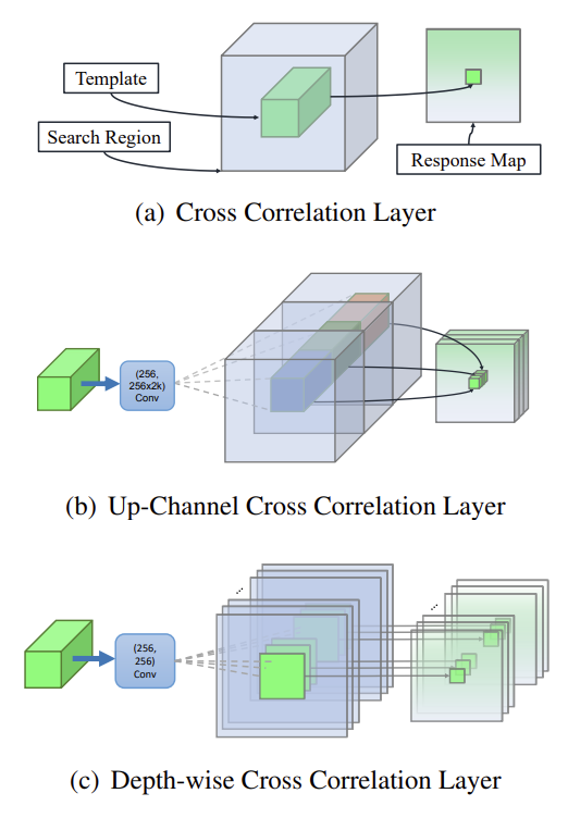
Fig 6. SiamRPN uses the up-channel cross correlation pictured in (b) whereas SiamRPN++ uses depth-wise cross correlation pictured in (c), significantly reducing the cross correlation channel size. [2].
Layer Wise Aggregation
The last major change they did was layer-wise aggregation. With a deeper feature extractor in the ResNet50, they had the ability to extract features from its different layers to fuse lower level feature information with higher dimensional features. As a result, the authors decided to extract the feature embeddings from conv3, conv4, and conv5 for more rich visual semantics that can help it identify target objects more robustly. Each output is thrown into a separate RPN and then the outputs of the RPN are combined through a weighted fusion layer to be used for bounding box regression and classification [2].

Fig 7. Features are extracted from the conv3, conv4, and conv5 blocks in the ResNet50 backbone and then fed into separate RPNs. Later on they are fused through a weighted sum. This is the layer wise aggregation process. [2].
Discussions
SiamRPN++ was able to reach SOTA on the VOT2018 benchmark on expected average overlap and accuracy. It was also near SOTA on the OTB-2015 dataset. However, since it is only a single object tracker, it has limitations in many applications. Additionally, it is not robust to new situations as you need to feed it the target frame in order for it to work. This can lead to increased computational complexity and memory consumption. Like many trackers, it also struggles with occlusions and has no clear solution for them. To address these issues, we looked into DeepSORT, an efficient multiple object tracker.
DeepSORT
The most popular tracking algorithm, DeepSORT, is applicable to many applications due to its efficient and robust nature. It utilizes an object detection network like YOLO to provide bounding boxes for each frame and a Kalman filter to take in previous detection data in order to predict the state of objects within the current frame. An association metric is used to measure the similarity of the predicted states and new object detections to assign the right detection to tracked objects. This is solved through what is called the Hungarian assignment problem.
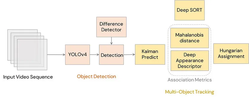
Fig 8. The architecture of DeepSORT using YOLOv4 as its detection model. [3].
In DeepSORT, each tracked object is assigned to a track. When a new object is detected on the frame, it is proposed to be assigned to a new track. Within the next three frames, the new proposed track has to be successfully associated with a measurement in order for the track to be added. Existing objects are all assigned to a single track which allows for easy identification and robustness to noisy measurement data in cases of occlusion, background clutter, and more. If there are no new measurements associated with an existing track after a certain number of timesteps, the track will be removed [3].
Kalman Filter
First, we should know how the different parts of DeepSORT work. One of the crucial parts is the Kalman Filter which basically takes in the previous state of an object and outputs a prediction of where it is going to be in the current time step (current frame). States of objects are represented in an 8d space \((u, v, \gamma, h, \dot{x}, \dot{y}, \dot{\gamma}, \dot{h})\) with (u, v) bounding box center coordinates, \(\gamma\) aspect ratio, h height, and their respective velocities. The Kalman filter takes in u, v, \(\gamma\), h as its direct observations and predicts the position and velocity of the object in the next frame. In DeepSORT, a constant velocity filter is used since the velocities between frames won’t change significantly. Detections from the YOLO model are used to update the state of the object and the prediction. With combined input coming from the YOLO model and the Kalman filter to track the object, you can adapt to noisy sensor data measurements such as occlusions while accounting for sudden changes in the object state [3].
Here is the Kalman Filter prediction implementation with constant velocity. Basically, the filter predicts where an object is going to be in the current time step given previous states and measurements.
def predict(self, mean, covariance):
    std_pos = [
        self._std_weight_position * mean[3],
        self._std_weight_position * mean[3],
        1e-2,
        self._std_weight_position * mean[3]]
    std_vel = [
        self._std_weight_velocity * mean[3],
        self._std_weight_velocity * mean[3],
        1e-5,
        self._std_weight_velocity * mean[3]]
    motion_cov = np.diag(np.square(np.r_[std_pos, std_vel]))

    mean = np.dot(self._motion_mat, mean)
    covariance = np.linalg.multi_dot((
        self._motion_mat, covariance, self._motion_mat.T)) + motion_cov

    return mean, covariance
Here is the Kalman Filter update step which is used to include information from new measurements in order to update the state of the object for future predictions.
def update(self, mean, covariance, measurement):
    projected_mean, projected_cov = self.project(mean, covariance)

    chol_factor, lower = scipy.linalg.cho_factor(
        projected_cov, lower=True, check_finite=False)
    kalman_gain = scipy.linalg.cho_solve(
        (chol_factor, lower), np.dot(covariance, self._update_mat.T).T,
        check_finite=False).T
    innovation = measurement - projected_mean

    new_mean = mean + np.dot(innovation, kalman_gain.T)
    new_covariance = covariance - np.linalg.multi_dot((
        kalman_gain, projected_cov, kalman_gain.T))
    return new_mean, new_covariance
Association Metric
The association metric determines how much new data observations align with the predicted states of different tracks. Using this metric, we can assign newly arrived states to existing tracks and update predictions accordingly. In DeepSORT, two types of metrics are used to determine the association: a Mahalanobis distance metric and an appearance metric based on a feature extractor. The Mahalanobis distance metric calculates the similarity between the motion information of predicted states and newly arrived measurements from the detection network. However, the distance metric on its own only works when motion uncertainty is low. Changes in camera angle and occlusions can make the Mahalanobis distance metric uninformed. This is why we add an appearance metric for more robust association [3].
Here is the code implementation for the distance metric:
def _pdist(a, b):
    a, b = np.asarray(a), np.asarray(b)
    if len(a) == 0 or len(b) == 0:
        return np.zeros((len(a), len(b)))
    a2, b2 = np.square(a).sum(axis=1), np.square(b).sum(axis=1)
    r2 = -2. * np.dot(a, b.T) + a2[:, None] + b2[None, :]
    r2 = np.clip(r2, 0., float(np.inf))
    return r2
For the appearance metric, DeepSORT uses a CNN architecture pre-trained on some dataset in order to develop well-discriminating feature embeddings. For example, you can train the CNN architecture on a person identification dataset. The architecture of the original CNN is provided in the table below. Each bounding box is thrown into the CNN to generate an appearance embedding for each proposed object. The appearance vector is then taken from the last layer of the CNN. For each track, we keep a history of the last 100 or so appearance associated descriptors and compare these with the appearance embeddings of new observations in order to find the most similar one using a cosine similarity [3].
| Name | Patch Size/Stride | Output Size |
|---|---|---|
| Conv1 | \(3 \times 3/1\) | \(32 \times 128 \times 64\) |
| Conv2 | \(3 \times 3/1\) | \(32 \times 128 \times 64\) |
| Max Pool 3 | \(3 \times 3/2\) | \(32 \times 64 \times 32\) |
| Residual 4 | \(3 \times 3/1\) | \(32 \times 64 \times 32\) |
| Residual 5 | \(3 \times 3/1\) | \($32 \times 64 \times 32\) |
| Residual 6 | \(3 \times 3/2\) | \(64 \times 32 \times 16\) |
| Residual 7 | \(3 \times 3/1\) | \(64 \times 32 \times 16\) |
| Residual 8 | \(3 \times 3/2\) | \(128 \times 16 \times 8\) |
| Residual 9 | \(3 \times 3/1\) | \(128 \times 16 \times 8\) |
| Dense 10 | \(128\) | |
| Batch and \(\mathcal{l}2\) normalization | \(128\) |
Table 1. Overview of the CNN architecture. [3].
The cosine similarity to calculate the distance between appearance vectors is implemented here:
def _cosine_distance(a, b, data_is_normalized=False):
    if not data_is_normalized:
        a = np.asarray(a) / np.linalg.norm(a, axis=1, keepdims=True)
        b = np.asarray(b) / np.linalg.norm(b, axis=1, keepdims=True)
    return 1. - np.dot(a, b.T)
Together these two metrics compliment each other to make more robust associations between predicted states of tracks and observations of the detection model. They are combined through a weighted sum producing the association between each track and each bounding box. The Mahalanobis distance metric is good for short term predictions based on motion while the cosine similarity of appearance information is good for long term behavior like when objects are occluded for a long time [3].
Hungarian Assignment
The Hungarian assignment is how bounding box detections are assigned to different tracks. Using the calculated associated metrics, we build a cost matrix where each column is a detected object and each row is a track. Therefore the \(i\) row and \(j\) column correspond to the association between the \(i\) track and \(j\) detection. A lower association metric (less distance between track and detection) means higher similarity. The Hungarian algorithm is then run on this matrix to determine an optimized matching that reduces the total cost. The results are stored in an assignment matrix where 1 in the \(i, j\) place of the matrix means a match between the \(i\) track and \(j\) detection. The corresponding information is used to update the Kalman prediction for more robust tracking. Unassigned detections are proposed to become new tracks. For the DeepSORT algorithm, more recently observed objects have higher precedence in matching then ones that haven’t been observed for a long time [3].
The algorithm for Hungarian assignment between new measurements and predicted states of tracks is given below:
def min_cost_matching(
        distance_metric, max_distance, tracks, detections, track_indices=None,
        detection_indices=None):
    if track_indices is None:
        track_indices = np.arange(len(tracks))
    if detection_indices is None:
        detection_indices = np.arange(len(detections))

    if len(detection_indices) == 0 or len(track_indices) == 0:
        return [], track_indices, detection_indices  # Nothing to match.

    cost_matrix = distance_metric(
        tracks, detections, track_indices, detection_indices)
    cost_matrix[cost_matrix > max_distance] = max_distance + 1e-5
    indices = linear_assignment(cost_matrix)

    matches, unmatched_tracks, unmatched_detections = [], [], []
    for col, detection_idx in enumerate(detection_indices):
        if col not in indices[:, 1]:
            unmatched_detections.append(detection_idx)
    for row, track_idx in enumerate(track_indices):
        if row not in indices[:, 0]:
            unmatched_tracks.append(track_idx)
    for row, col in indices:
        track_idx = track_indices[row]
        detection_idx = detection_indices[col]
        if cost_matrix[row, col] > max_distance:
            unmatched_tracks.append(track_idx)
            unmatched_detections.append(detection_idx)
        else:
            matches.append((track_idx, detection_idx))
    return matches, unmatched_tracks, unmatched_detections
Discussions
DeepSORT is increasingly robust to occlusions due to its Kalman filter that can predict states even when there are noisy observations for an object. It also provides computationally efficient and easy implementation for multiple object tracking, making it widely used in many cases. However, a bottleneck of the algorithm is the object detector. A bad object detector will degrade performance and lead to tracking failures and drift. Additionally, it may be hard to track objects in low illumination and when there are other factors that can affect the detection performance. DeepSORT is also not very scalable as it relies on pretrained architectures to do feature extraction and detection. Because it also only takes into account appearance and motion information, it can be susceptible to performance degradation when non-rigid transformations occur [3].
ODTrack
ODTrack (Online Dense Temporal Token Learning for Visual Tracking) is a new framework designed for video-level object tracking.
Some of the problems associated with object tracking is that traditional methods only cover a limited number of frames which fail to capture long term dependencies across the videos. If objects are obscured by other objects, the frame by frame analysis has difficulty re-identifying them once they reappear in a new frame. If objects undergo changes in size or shape throughout a video, traditional frameworks may struggle to track the object from information from a single frame. ODTrack aims to address these problems [4].
Core functionalities:
Online tokenization: ODTrack processes the entire video as a whole instead of analyzing each frame independently and then extracts the features about the object’s appearance from each frame which are then compressed into a sequence of tokes.
Temporal Information Capture (How the object moves across frames): ODTrack employs online token propagation which iteratively updates the token sequence across video frames which allows it to capture the object’s motion patterns.
Frame-to-Frame Association: ODTrack can effectively associate the object between frames which allows it to track the object’s movement throughout the entire video [4].
Architecture:
Feature Extraction Backbone:
- Where ODTrack processes each frame of the video
- Uses pretrained model to extract features from each frame
Tokenization Module:
- The information from the features are fed into the tokenization module which compresses the features into a sequence of tokens
- With the changes of the video, it refines the token sequence to incorporate the information of the objects changed appearance and motion across frames
Frame-to-Frame Association Module:
- Takes the last
Pros:
Simplicity and Efficiency: This is a much more streamlined approach with online token propagation allowing for computational efficiency.
Effective Long-term Dependency Capture: ODTrack has the ability to capture these long-term dependencies through the propagated token sequence which leads to more accurate tracking. This also makes the framework very flexible to handle videos of various lengths, qualities, and scenarios [4].
Cons:
Information Loss: Compressing information into tokens can lead to loss of detail which may cause some discrepancies in the object characteristics for tracking.
New: ODTrack is a relatively new framework so it may not be as tested as other traditional methods, so there is lots of room to improve.
Demo
Code Base: Github
As you can see there are multiple boxes within each frame surrounding the multiple objects in the video. DeepSORT is also robust to camera movement as the demo videos show. These demo videos are pretty clear and not noisy so it remains to be seen if DeepSORT can have similar performance with more noisy data.
Conclusion
For single object tracking tasks, SiamRPN++ is a great option that isn’t computationally expensive and is very accurate when you want to optimize for a specific tracking environment. Additionally, the one shot learning task minimizes online training. In comparison, DeepSORT is a better option when you want to generalize to many different domains, environments, and scenarios due to its multiple object tracking structure, ability to track through noisy camera data, and efficiency. However, the detection model and appearance extractor may need fine-tuning which requires more online training. Each tracking algorithm has their own benefits and are useful in different situations which is why both are still widely used today. ODTrack is also a solid option for computational efficiency and robustness to different tracking scenarios.
Reference
[1] Li, Bo, et al. “Siamrpn++: Evolution of siamese visual tracking with very deep networks.” Proceedings of the IEEE/CVF conference on computer vision and pattern recognition. 2019.
[2] Li, Bo, et al. “High performance visual tracking with siamese region proposal network.” Proceedings of the IEEE conference on computer vision and pattern recognition. 2018.
[3] Wojke, Nicolai, Alex Bewley, and Dietrich Paulus. “Simple online and realtime tracking with a deep association metric.” 2017 IEEE international conference on image processing (ICIP). IEEE, 2017.
[4] Zheng, Yaozong, et al. “ODTrack: Online Dense Temporal Token Learning for Visual Tracking.” arXiv preprint arXiv:2401.01686 (2024).