Trajectory Prediction
In the AV pipeline, trajectory prediction plays a crucial role in the Autonomous Vehicle (AV) pipeline. In this report we’ll explore two different machine learning approaches to trajectory prediction for Autonomous Vehicles: a Conv-based architecture which uses rasterized semantic maps, and a GNN-based architecture which uses a vector-based representation of the scene.
Introduction
Trajectory prediction is the process of predicting the future positions of agents over time. Specifically, given a series of \(t\) previous frames, each containing the locations and classes of \(n\) actors, the goal of a trajectory prediction algorithm is to be able to predict the locations of all agents for frame \(t+1\). For Autonomous Vehicles, having an accurate trajectory prediction algorithm is incredibly important as it allows AVs to predict the movement of road-agents (i.e. other vehicles, pedestrians, etc.), and adjust its route accordingly to avoid accidents. Trajectory prediction is difficult because it often requires a holistic understanding of the scene and its actor interactions.
ConvNet
A common way to tackle the problem is to encode the scene as a rasterized HD semantic map. This is typically done by taking the classified actors extracted from the AV’s perception system and overlaying their locations and class attributes on top of a bird’s eye view of the scene. This lets us treat the problem as a computer vision task, as we can then feed these maps into a Convnet-based architecture like ResNet. One advantage of this approach is that this allows for the use of various pretrained vision models, where the backbone can be used as a feature extractor.
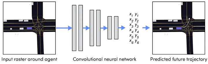
Fig 1. A deep learning-based approach to trajectory prediction [1].
Instead of class predictions, the model returns \(n\) pairs of values, where each pair represents the predicted future (x,y) location of a target, and \(n\) represents the number of future frames to predict. The loss is simply calculated to be the Mean Squared Error (MSE) between the locations of the predicted and actual values of agents:
\[L(x, x_p) = \frac{1}{n} \sum_{i}^{n} (x - x_p)^2\]where \(x\) and \(x_p\) can be either the x or y coordinate of each agent location at a given frame.
Implementation
To see this model in action, we ran Woven Planet’s prediction notebook, which uses the Lyft’s Level 5 Self-driving motion prediction dataset [2] for training. While Woven’s notebook uses a pretrained ResNet model as the backbone, we decided to experiment using an EfficientNet instead. EfficientNet utilizes a technique called compound-coefficient to scale up models efficiently [3], which is especially useful given the scale of Lyft’s dataset. The following code snippet shows how the EfficientNet backbone is implemented. Note how the first and last layer is modified in order to accommodate the input and output shape:
class EfficientNet(nn.Module):

    def __init__(self):
        super().__init__()

        # replace first and last layer to match shape of data
        self.model = efficientnet_b0(pretrained=True)
        num_history_channels = (cfg["model_params"]["history_num_frames"] + 1) * 2
        in_channels = 3 + num_history_channels
        self.model.features[0] = Conv2dNormActivation(
            in_channels,
            self.model.features[0].out_channels,
            kernel_size=3,
            stride=2,
            norm_layer=nn.BatchNorm2d,
            activation_layer=nn.SiLU
        )
        # num future states * x, y coordinates
        num_targets = 2 * cfg["model_params"]['future_num_frames']
        self.model.classifier[1] = nn.Linear(in_features=self.model.classifier[1].in_features, out_features=num_targets)

    def forward(self, x):
        x = self.model(x)
        return x

    def to(self, device):
        return self.model.to(device=device)
Results
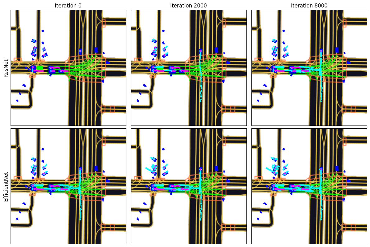
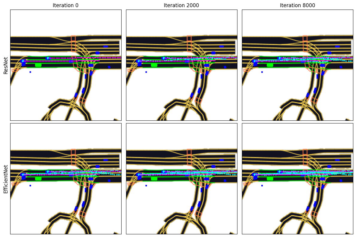
Fig 2. Visualizations of Resnet and Efficientnet performance during training. The cyan dots represents the model’s predicted location, while the purple dots represents the ground truth locations.
From the visualizations above, we see that the Resnet and Efficientnet models are both able to predict the general path of each agent. However, Efficientnet was able to train the same number of iterations as Resnet in about a third of the time.
VectorNet
One drawback that CNN-based architectures have is their relatively high memory and performance requirements, which is a key factor for Autonomous Vehicle systems as they require real-time calculations. VectorNet was designed to overcome those issues by encoding the environment in a graph-based system [4].
Architecture
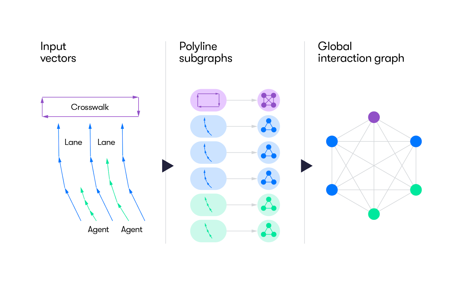
Fig 3. Vectornet Pipeline [4].
VectorNet is a hierarchical GNN (graph neural network) that processes environment and agent dynamics through two main stages. It uses Local Graphs to process individual road components, such as lanes and traffic lights, as well as agents like pedestrians and other cars. It uses a Global Interaction Graph to model higher-order interactions among all of these smaller agents such as how pedestrians and cars might interact, or how cars would interact with each other at a 4-way stop.
Vectorized Representation
The architecture of VectorNet is unique in how it takes in input and transforms it into something very efficient for a machine learning model to use. VectorNet takes in high-definition maps as input. Where other previous architectures have taken these HD maps and interpreted them using color-coded agent extraction where they then feed them into CNNs, VectorNet takes a different approach. Researchers at Waymo understood that interpreting HD maps in that way caused a limited receptive field, so they decided to learn a meaningful context representation directly from the well-structured HD maps. Using points, polygons, and curves in geographic coordinates, they represented all sorts of agents as geometric polyline defined by multiple control points.
The reason VectorNet uses polylines to represent the input is because remapping the input (a set of pixels with colors and brighnesses) as vectorized lines prevents any sort of information loss about direction and speed of agents all the while making sure that the input is fed in a very computationally efficient way.
Local Graphs
Then, each polyline representing road elements or agents on the road is processed in a local graph to capture spatial structure and attributes. The way the researchers in VectorNet do is is by using multi-layer perceptrons (MLPs) to encode each vector (which represents a node in this local graph) within a polyline. Then, they use max pooling to aggregate information within these polylines. In doing so, they are able to capture local context and relationships between points belonging to the same polyline.
Global Interaction Graph
Now that they have finished encoding local information within the polyline, VectorNet then constructs this novel architecture element called a global interaction graph. A global interaction graph is a graph where each node is an entire polyline and the edges between nodes are the interactions between polylines. In doing so, researchers are able to capture the high-order interactions among all the road elements and agents represented by polylines. This graph is a fully connected graph ans employs the self-attention mechanism in order to model all the complex interactions between nodes. The output features of this graph are then used for downstream tasks like trajectory prediction.
Auxiliary Task for Contextual Learning
An auxiliary task that is mentioned in the VectorNet paper is the use of masking. This auxiliary task is where researchers randomly mask parts of the input data (whether it is map features or agent trajectories) and attempt to recover these items while training. This is a form of self-supervised learning and encourages the model to learn richer context representations. During training, a subset of the input node features, which could represent elements of the HD maps (e.g., lanes, traffic signs) or dynamic elements like agent trajectories, are randomly selected and masked out. The masking is implemented by setting the features of these selected nodes to zero or replacing them with a special token that indicates missing information. Thus, the final objective function of the model is:
\[L = L_{\text{traj}} + \alpha L_{\text{node}}\]Where \(L_{\text{traj}}\) represents the negative Gaussian log-likelihood for the predicted trajectories, and \(L_{\text{node}}\) represents the Huber loss for predicting masked node features.
Performance
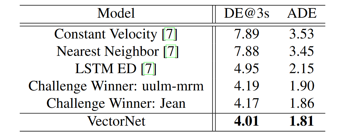
Fig 4. Trajectory prediction performance on the Argoverse Forecasting test set [4].
The trajectory prediction capabilities of autonomous vehicle (AV) systems are benchmarked against metrics that reflect their precision and efficiency in real-world scenarios. VectorNet stands out in this domain, as illustrated by both its ADE (Average Displacement Error) and DE@3s metrics, which demonstrate its exceptional ability to predict the future positions of on-road agents. It boasts an ADE of 1.81 meters, showcasing superior average accuracy across time steps, and a DE@3s of 4.01 meters, highlighting its precision in short-term trajectory forecasting. This performance surpasses traditional approaches like constant velocity models and LSTM-based architectures, which were once standard.
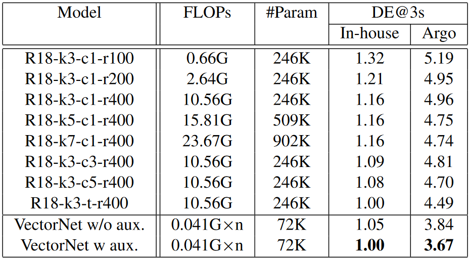
Fig 4. FLOPs and param # for Vectornet compared with other Resnet models [4].
Vectornet also outperforms other Resnet models in terms of FLOPs and the number of parameters. This is crucial for AV systems that must operate within strict computational constraints.
References
[1] Woven Planet Level 5. (2021, October 25). How to build a motion prediction model for Autonomous Vehicles. Medium. https://medium.com/wovenplanetlevel5/how-to-build-a-motion-prediction-model-for-autonomous-vehicles-29f7f81f1580
[2] Houston, John, et al. “One Thousand and One Hours: Self-driving Motion Prediction Dataset.” CoRR. 2020.
[3] Tan, Mingxing & Le, Quoc. “EfficientNet: Rethinking Model Scaling for Convolutional Neural Networks.” International Conference on Machine Learning. 2019.
[4] Gao, Jiyang, et al. “VectorNet: Encoding HD Maps and Agent Dynamics from Vectorized Representation.” Conference on Computer Vision and Pattern Recognition. 2020.