Deep Learning for Prostate Segmentation

We aim to analyze how we can use deep learning technique for prostate image segmentation. Prostate cancer is the second most common form of cancer for men worldwide and the fifth leading cause of death for men globally [3]. However, this is a statistic that can be considerably changed with early stage detection. In fact, the cancer is completely curable within 5 years if we catch it early. To this end, we explore how we can use existing deep learning architectures to help with prostate image segmentation to catch early prostate cancer in patients.

• History
• Enter Deep Learning
• Models
  • ENet
  • UNet
• Model Comparison
• Conclusion
• References

History

Classical approaches to 3D image generation of inner tissues and organs involved manual delineation/contouring which were incredibly time-consuming, expensive and had rigid calculations for irregular shapes which led to inaccurate measurements. Traditional statistical models such as K-Means, SVMs and Random Forest were just as inaccurate since they depended on handcrafted features and required significantly more preprocessing.

Enter Deep Learning

We can think of prostate segmentation as classifying voxels as either part or not part of a tumor. We then use prior training examples to understand how model boundaries of prostate in a “noisy advantage”. This has a dual advantage of performing image classification and segmentation simultaneously, reducing overhead, leading to faster diagnoses. The lowered costs and increased speeds such methods provide also increases accessibility to prostate cancer detection methods in emerging economies where medical infrastructure is substandard.

Models

ENet

ENet is a fast and compact Encoder-Decoder network. The vanilla ENet model assumes an input size of \(512 \times 512\). The initial ENet block has a convolution operation (\(3 \times 3\), stride 2), max pooling, then a concatenation. The convolution has 13 filters, which produces 16 feature maps after concatenation. Then comes the bottleneck module. Here, convolution is either regular, dilated or full with \(3 \times 3\) filters, or a \(5\times5\) convolution into asymmetric ones. Then using a skip connection, merge back with element-wise addition. There is also Batch Normalization and PReLU between all convolutions. The below Figure 1 highlights the overall model architecture.

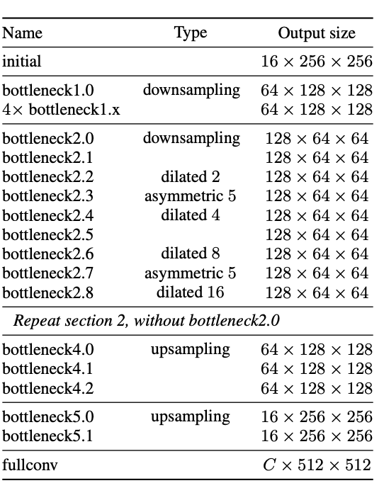
Fig 1.ENet: An object Segmentation Method [2].

1. Feature Map Resolution: There are two main issues with downsampling during image segmentation. Reducing image resolution means the loss of exact edges and very strong downsampling will require just as strong upsampling, which is costly and inefficient. ENet addresses these concerns by adding the feature maps produced by the encoder and saving the indices that were chosen in max pooling layers to be later formed as upsampled maps in the decoder.

2. Early Downsampling: Processing large input frames is very expensive, and this occurs mainly at the lower blocks of the model. ENet’s first two blocks heavily reduce the input size and use a small amount of feature maps. This works since visual information is normally very redundant, so compressing it makes operations much more efficient.

3. Early Downsampling: Processing large input frames is very expensive, and this occurs mainly at the lower blocks of the model. ENet’s first two blocks heavily reduce the input size and use a small amount of feature maps. This works since visual information is normally very redundant, so compressing it makes operations much more efficient.

4. Dilated Convolutions: It is very important for the model to have a wide receptive field, so to avoid overly downsampling, dilated convolutions replace the main convolutions inside the bottlenecks. They did this for the stages that operate on the smallest resolutions. The best accuracy was obtained when these convolutions were combined with other bottleneck modules.

5. Regularization: Regularization techniques are vital for enhancing the performance and generalization capability of UNet, a neural network architecture widely used for tasks like image segmentation. Dropout, which randomly deactivates units during training, can be applied to convolutional layers in both the contracting and expansive paths to discourage over-reliance on specific features. Weight decay, or L2 regularization, penalizes large weights in the network’s parameters, promoting simpler models and preventing overfitting. Data augmentation, involving transformations like rotation and flipping, diversifies the training data, aiding in better generalization. Batch normalization normalizes layer activations, accelerating training and acting as a form of regularization by reducing internal covariate shift. Finally, early stopping halts training when validation loss starts increasing, preventing overfitting and encouraging the model to learn more generalizable patterns. These techniques, either individually or combined, play a crucial role in optimizing the performance and robustness of UNet models for various applications. In the original ENet paper, spacial dropout showed the best results in order to prevent overfitting of the pixel-wise datasets, which tend to be quite small [2].

ENet’s main advantage is its speed. It can achieve surprisingly high accuracy while using computational resources very sparingly and working very quickly. This is why it was initially developed for real-time applications, such as self driving cars. It was later adapted to other uses, such as medical image segmentation, which is of use to us when detecting prostate cancer.

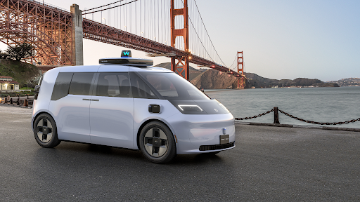
Fig 2. A self-driving car that could perhaps be making use of ENet.

UNet

UNet was developed specifically for biological image segmentation. Now, UNet’s architecture is distinctive with distinct dual pathways: the contracting and expansive paths. The contracting path, comprising encoder layers, captures context and diminishes input spatial resolution. Conversely, the expansive path, housing decoder layers, deciphers encoded data using skip connections from the contracting path to produce a segmentation map.

In the contracting path, relevant features are discerned from the input image. Encoder layers execute convolutions, reducing spatial resolution while deepening feature maps to abstract representations. This process mirrors feedforward layers in conventional CNNs. Conversely, the expansive path decodes encoded data, retaining input spatial resolution. Decoder layers upsample feature maps and perform convolutions, aided by skip connections to restore spatial information lost during contraction, facilitating more precise feature localization.

Distinct features of UNet:

1. \(3 \times 3\) convolutions -> \(5 \times 5\) convolutions: consider more information in each step
2. 0 padding the input: ensure size of output feature maps = size of input
3. Input size of \(512 \times 512\)
4. 32 filters in first layer of encoder -> produces 32 feature maps: fine-grained details in image captured from beginning
5. Doubled the feature maps after each max pooling layer, which halves dimensions of the map itself, clamping at 256 feature maps (each feature map has dimensions of \(64 \times 64\) here): focus on most prominent/distinct features and capture more abstract representation Normalization of the scale of data to prevent large weights: prevents overfitting + faster convergence

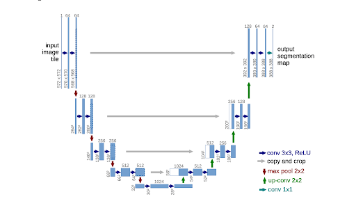
Fig 3. UNET Architecture [1].

Training Methodology

UNet features 5-fold cross validation to prevent overfitting (68 in train set, 17 in test). It uses the Tversky loss function, which features an adapted version of the Dice Score Coefficient (DSC) to account for various data imbalance. In the original paper, experiments found that 0.00001 was the most optimal learning rate while the constants \(\alpha = 0.3\), \(\beta = 0.7\), \(N = 8\) were used for Tversky Loss.

Fig 4. Mathematical equations used in the loss function.

Model Comparison

ENet and UNet are both widely used architectures for image segmentation, each with its own strengths and characteristics. ENet, known for its efficiency and lightweight design, features a simple encoder-decoder structure with skip connections, making it suitable for real-time applications on resource-constrained devices. In contrast, UNet is a more complex architecture specifically designed to capture both local and global features effectively, particularly in biomedical image segmentation tasks like prostate segmentation.

When comparing the two models, ENet typically has fewer trainable parameters and a smaller size on disk compared to UNet, indicating a simpler architecture that requires less storage space. Furthermore, ENet demonstrates significantly lower inference times on both CPU and GPU, making it highly efficient for processing images in real-time scenarios. These advantages make ENet an attractive option for tasks where computational efficiency is paramount.

Model Name	Trainable Parameters	Non-Trainable Parameters	Size on Disk	Inference Time/Dataset (CPU)	Inference Time/Dataset (GPU)
ENet	362,992	8,352	5.8 MB	6.17 s	1.07 s
UNet	5,403,874	0	65.0 MB	42.02 s	1.57 s

However, for prostate image segmentation, where precise delineation of structures is crucial, UNet may be preferred despite its higher computational cost. UNet’s deeper layers and skip connections enable it to capture fine details and contextual information more effectively, leading to better segmentation accuracy. In tasks like medical image segmentation, where accuracy is paramount, the improved performance of UNet outweighs its higher computational demands.

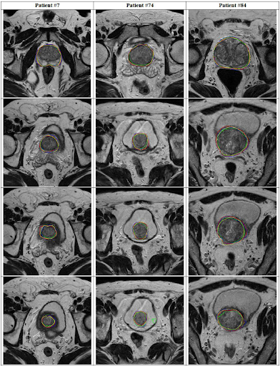
Fig 5. Segmentation comparison: yellow is manual, red is ENet, green is UNet.

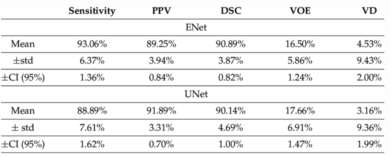
Fig 6. A more detailed model comparison. [4]

In summary, while ENet offers superior efficiency and speed, UNet’s architecture is better suited for complex segmentation tasks like prostate image segmentation, where achieving high accuracy and detail preservation is essential, even at the cost of increased computational resources.

Conclusion

We believe UNet is the best model for prostate segmentation. While it might carry an overhead in processing times and a much larger GPU footprint making it significantly more expensive to train and deploy, we believe the fact that it has a significantly higher number of trainable parameters make it perfect for complex use cases, which are critical in detecting early stage prostate cancer. This also means that the number of false positive disease diagnosis will fall significantly along with the far more dangerous false negatives.

References

[1] Zhang, Jeremy. “UNet – Line by Line Explanation.” Towards Data Science, https://towardsdatascience.com/unet-line-by-line-explanation-9b191c76baf5/. 2019.

[2] Paszke A; Chaurasia A; Kim S; Culurciello E. “ENet: A Deep Neural Network Architecture for Real-Time Semantic Segmentation.” arXiv 2016, arXiv:1606.02147.

[3] “Key Statistics for Prostate Cancer | Prostate Cancer Facts.” American Cancer Society, www.cancer.org/cancer/types/prostate-cancer/about/key-statistics.html#:~:text=About%201%20in%208%20men.

[4] Comelli, Albert, et al. “Deep Learning-Based Methods for Prostate Segmentation in Magnetic Resonance Imaging.” Applied Sciences, vol. 11, no. 2, 15 Jan. 2021, p. 782, https://doi.org/10.3390/app11020782.

---