Text-to-Video Generation
In this paper, we will discuss diffusion-based video generation models. We will first do a preliminary exploration of diffusion, then extend it to video generation by examining Video Diffusion Models by Jonathon Ho, et al. We will then follow this with a refinement of video diffusion models by conducting a deep dive into Imagen Video, a high definition video generation model developed by researchers at Google. Through this paper, we aim to provide an overview of diffusion-based video generation, as well as rigorously cover a high definition refinement of the basic video diffusion model.
- Introduction
- Diffusion
- Video Diffusion Models
- Imagen Video
- Loss Function
- Experiments
- Comparison
- Reference
Introduction
Text to video generation is a computer vision task that uses deep learning to create a video from a text description. It takes an input of a text script, like a story or description and ideally outputs a high definition video that encapsulates the content of the script. It uses natural language prompts to understand the content of the text for the video output. Here is an example using Sora, a video generation model developed by OpenAI:
Fig 1. Prompt: The camera directly faces colorful buildings in Burano Italy. An adorable dalmatian looks through a window on a building on the ground floor. Many people are walking and cycling along the canal streets in front of the buildings. [5]
Diffusion
Forward Diffusion Process
In diffusion, the forward process entails the adding of noise to the datapoint. Diffusion models usually sample this noise from a Gaussian distribution according to a noise schedule, but other distributions are possible. Diffusion models usually have a Markov Chain structure (meaning that future events only depend on the current state). By the end of the process, the datapoint should resemble the Gaussian noise, while maintaining key features of the image, allowing for the backward process to detect and utilize those features to reconstruct the whole image.It is typical to use a cosine noise schedule which has this Markov structure:
\[q(\mathbf{z}_t|\mathbf{z}_s) = \mathcal{N}(\mathbf{z}_t; (\alpha_t/\alpha_s)\mathbf{z}_s, \sigma^2_{t|s}\mathbf{I})\]Backward Diffusion Process
The backward process can be understood as running the forward diffusion process in the other direction. Starting with a very noisy image, the idea to sample noise from a Gaussian distribution and progressively remove this noise from the image until the original image has been reconstructed. The reverse process aims to learn the conditional distribution \(p*\theta (\mathbf{x}*{t-1} | \mathbf{x}\_t)\) which represents the noise we need to subtract from the order at time t in order to obtain the image at time t-1.
Video Diffusion Models
3D U-Net
This architecture modifies the original U-Net by substituting the 2D convolution with a space-only 3D convolution. Specifically, a conventional 3x3 convolution is replaced by a 1x3x3 convolution. Here, the first dimension represents the video frame (i.e., the time dimension), while the second and third dimensions correspond to the frame height and width, respectively (i.e., the spatial dimensions). Given that the first dimension is set to 1, it does not affect the temporal aspect but solely impacts the spatial dimensions. The architecture retains the spatial attention block, where attention is exclusively applied to the spatial dimensions, effectively treating the time dimension as part of the batch dimension. Following each spatial attention block, a new temporal attention block is introduced. This block focuses on the time dimension for attention, merging the spatial dimensions into the batch dimension for processing.
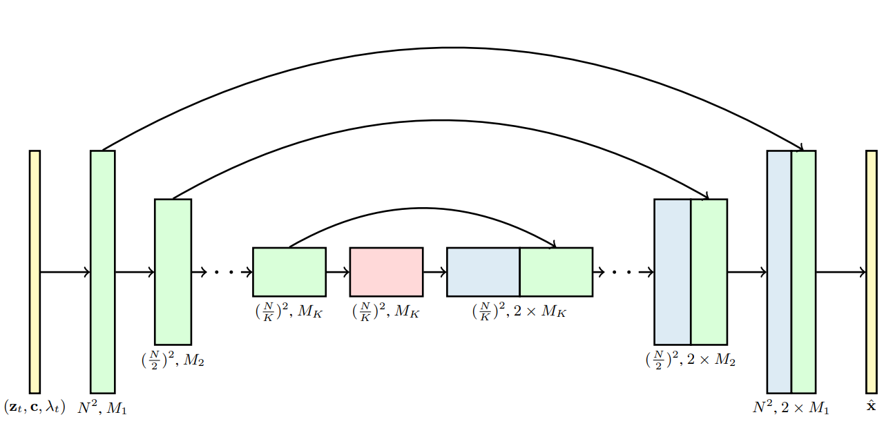
Fig 2. The 3D U-Net architecture for xˆθ in the diffusion model. Each block represents a 4D tensor with axes labeled as frames × height × width × channels, processed in a space-time factorized manner as described in Section 3. The input is a noisy video zt, conditioning c, and the log SNR λt. The downsampling/upsampling blocks adjust the spatial input resolution height × width by a factor of 2 through each of the K blocks. The channel counts are specified using channel multipliers M1, M2, …, MK, and the upsampling pass has concatenation skip connections to the downsampling pass [1]
In addition, we use relative position embeddings in each temporal attention block so that the network can distinguish the order of video frames without relying on the specific video frame time. This method of first performing spatial attention and then performing temporal attention can be called factorized space-time attention.
Video-Image Joint Training Video Diffusion
One advantage of using factorized space-time attention is that we can implement the video-image joint training.
To implement this, random independent image frames are concatenated to the end of each video sampled from the dataset. Attention in the temporal attention blocks is masked to prevent the mixing of information across video frames and each individual image frame. These random independent images are selected from various videos within the same dataset.
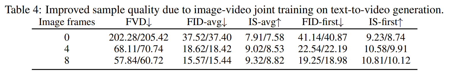
Fig 3: showcases results from an experiment on text-conditioned videos (16x64x64), where training included an additional 0, 4, or 8 independent image frames per video. The data reveal significant enhancements in quality metrics for both video and image samples as the number of added frames increases. Adding these frames reduces gradient variance, introducing a slight bias in the video modeling objective but effectively optimizing memory use by allowing more independent examples per batch.
Autoregressive Video Extension for Longer Sequences
The Video Diffusion Models paper also introduces a method for generating extended video sequences using an autoregressive process. This approach enables the model to predict subsequent frames based on previously generated ones. This allows the model to effectively create videos of arbitrary lengths. To improve the temporal coherence between frames in extended videos, the paper proposes reconstruction-guided sampling. The method demonstrates significant improvements over previous techniques for generating extended length videos.
Examples of Video Diffusion
Fig 3. Examples from Video Diffusion Models [1]
Imagen Video
Imagen Video is a video-generation system based on a cascade of video diffusion models. It consists of 7 sub-models dedicated to text-conditional video generation, spatial super-resolution, and temporal super-resolution. Imagen video has the capacity to generate high definition videos (1280x768) at 24 frames per second for a total of 128 frames.
Loss Function
This model is trained using the below loss function
\[\mathcal{L}(\mathbf{x}) = \mathbb{E}_{\mathbf{\epsilon} \sim \mathcal{N}(0,\mathbf{I}), t \sim \mathcal{U}(0,1)} \left[ \| \hat{\mathbf{\epsilon}}_{\theta}(\mathbf{z}_t, \lambda_t) - \mathbf{\epsilon} \|_2^2 \right]\]Cascaded Architecture:
Cascaded Diffusion Models, introduced by Ho et al. in 2022, have emerged as a powerful technique for generating high-resolution outputs from diffusion models, achieving remarkable success in diverse applications such as class-conditional ImageNet generation and text-to-image creation. These models operate by initially generating an image or video at a low resolution and then progressively enhancing the resolution through a sequence of super-resolution diffusion models. This approach allows Cascaded Diffusion Models to tackle highly complex, high-dimensional problems while maintaining simplicity in each sub-model.
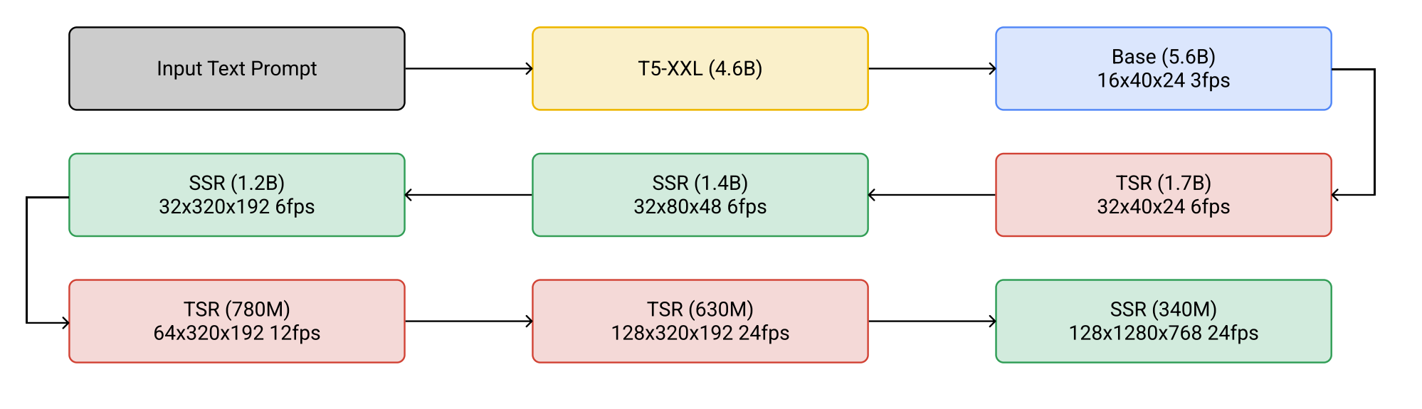
Figure 2: The cascaded sampling pipeline starting from a text prompt input to generating a 5.3- second, 1280×768 video at 24fps. “SSR” and “TSR” denote spatial and temporal super-resolution respectively, and videos are labeled as frames×width×height. In practice, the text embeddings are injected into all models, not just the base model. [2].
The figure above summarizes the entire cascading pipeline of Imagen Video:
- Text encoder : Encode text prompt to text_embedding
- Base video diffusion model
- SSR*3 (spatial super-resolution): increase spatial resolution for all video frames
- TSR*3 (temporal super-resolution): increase temporal resolution by filling in intermediate frames between video frames
SR3: Mechanism of Super-Resolution Block:
The SSR (Super-Resolution via Repeated Refinement) and TSR blocks implement a mechanism for conditional image generation known as SR3. This method revolves around training on sets that comprise pairs of low-resolution (LR) and high-resolution (HR) images. The inputs for training include:
- A low-resolution image, denoted as x
- Noisy image yt, which is derived from High-Resolution image y0 using the equation \(\bar{y}=\sqrt{\gamma}y_0+\sqrt{1-\gamma}\epsilon\)
- Noise variance $\gamma$, which correlates with the total number of training step T.
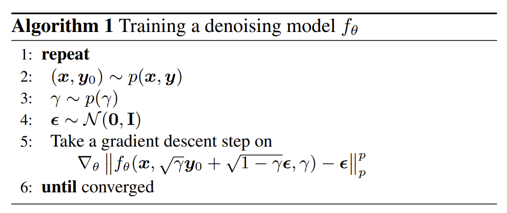
Fig 3: Algorithm for diffusion.[3]
Remark: The meaning of the loss function here is to make the difference between the noise output by the model and the randomly sampled Gaussian noise as small as possible.
Inference Process:
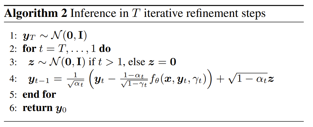
Fig 4: Algorithm for iterative refinement.
The process begins with a low-resolution image x and a noisy image yt containing Gaussian noise, aiming to output a high-resolution image. This input undergoes T iterations of a specific formula to produce a super-resolution (SR) image. This procedure can be seen as progressively eliminating noise from the image. With sufficient iterations, noise is effectively removed, resulting in an enhanced super-resolution image.
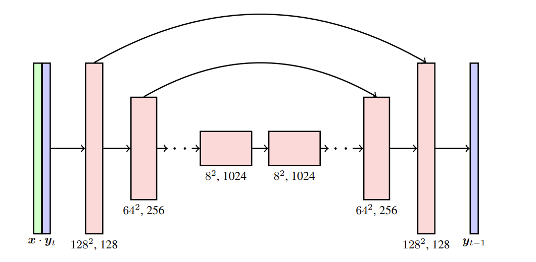
Fig 5: Description of the U-Net architecture with skip connections. The low resolution input image x is interpolated to the target high resolution, and concatenated with the noisy high resolution image yt. We show the activation dimensions for the example task of 16×16 → 128×128 super resolution.[4]
Spatial Super-Resolution:
Use bilinear interpolation to upsample a low-resolution video (such as 32 x 80 x 48) to a high-resolution video (such as 32 x 320 x 192) x, then concatenate x with the noisy high-resolution video yt in the channel dimension as the input data of U-Net.
Temporal Super-Resolution:
Upsample a low frame number video (such as 32 x 320 x 192) to a high frame number video (such as 64 x 320 x 192) x by inserting blank frames or repeated frames. Then concatenate x with the noisy high-frame video yt in the channel dimension as the input data of U-Net.
V-Prediction
Instead of using conventional \(\epsilon\)-prediction to add noise, the author introduces a new technique known as velocity prediction parameterization, or v-prediction, for the video diffusion model. This method is summarized by the prediction formula \(v\equiv\alpha_t\epsilon-\sigma_tx\), leading to \(\hat{x}=\alpha_tz_t-\sigma_t\hat{v}_\theta(z_t)\).
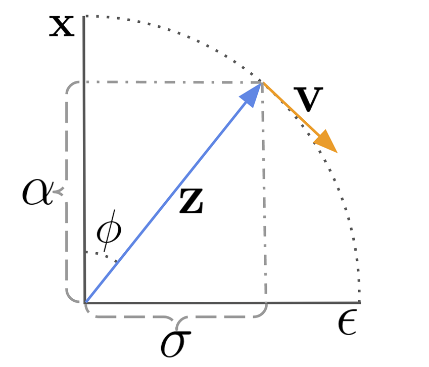
Fig 6: Visualization of reparameterizing the diffusion process in terms of and \(v\) and \(v_\phi\).[4]
Let’s delve into the derivation of the first equation. Remember the noise addition equation in DDPM:
\[x_t=\sqrt{\bar{a}_t}x_0+\sqrt{1-\bar{a}_t}\epsilon \hspace{1cm} (1)\]where the sum of the squares of the coefficients of \(x_0\) and \(\epsilon\) equals 1. This allows for a substitution using sine and cosine. The paper adopts the noise addition equation
\[z_t=\alpha_tx+\sigma_t\epsilon \hspace{1cm}(2)\]Before proceeding with the derivation, it’s important to align our symbols: in equation (1), \(x\) represents \(x_0\), while \(\alpha_t\) and \(\sigma_t\) correspond to \(\sqrt{\bar{a}_t}\) and \(\sqrt{1-\bar{a}_t}\), respectively. Also, \(z_t\) in equation (2) represents \(x_t\) in equation (1).
Defining \(\alpha_\alpha=\cos(\phi)\) and \(\sigma_\alpha=\sin(\phi)\), we obtain \(z_{\phi} =\cos(\phi)x+\sin(\phi)\epsilon\). Taking the derivative of \(z\) with respect to \(\phi\), we find the velocity equation:
\[v_{\phi} =\frac{d z_{\phi}}{d\phi}=\frac{d\cos(\phi)}{d\phi}x+\frac{d\sin(\phi)}{d\phi}\epsilon=\cos(\phi)\epsilon-\sin(\phi)x =\alpha_{\phi}\epsilon-\sigma_{\phi}x \hspace{1cm} (3)\]Next, we apply \(\alpha_t\) to both sides of equation (2) and \(\sigma_t\) to both sides of equation (3), resulting in: \(\sigma v=\alpha \sigma \epsilon- \sigma^2 x\), and \(\alpha z=\alpha^2 x+\alpha \sigma \epsilon\). Subtracting these two equations cancels the term \(\alpha \sigma \epsilon\), yielding: \(\sigma v-\alpha z=-\sigma^2 x-\alpha^2 x= -(\sigma^2+\alpha^2)x\). Given that the sum of the squares of these two terms equals 1, we conclude with \(\hat{x}=\alpha_tz_t-\sigma_t\hat{v}_\theta(z_t)\).
Remark: Similar to \(\epsilon\)-prediction, v-prediction introduces noise to the samples during the training process. However, when calculating the MSE loss function, velocity is used in place of \(\epsilon\).
In the context of video diffusion model training, the author highlights the following advantages of v-prediction:
- It significantly enhances numerical stability throughout the diffusion process, facilitating progressive distillation.
- It prevents the temporal color shifting often observed in models using $\epsilon$-prediction.
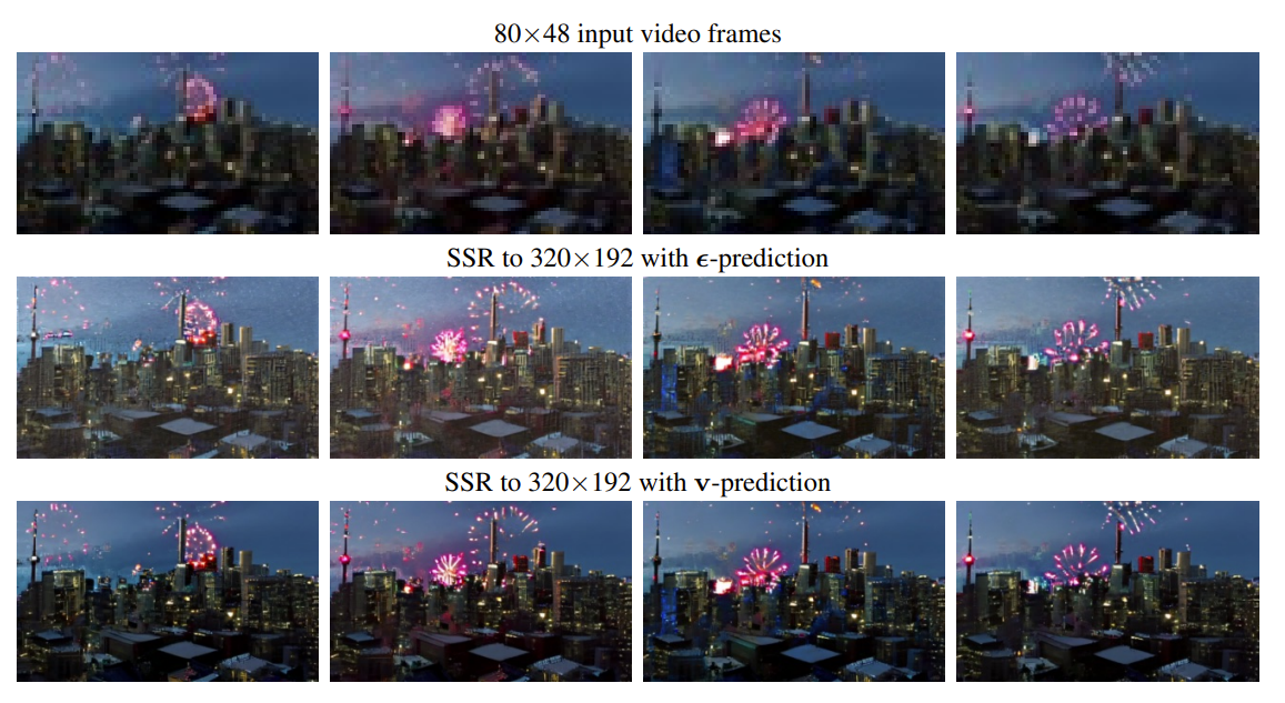
Fig 6: Comparison between \(\epsilon\)-prediction (middle row) and v-prediction (bottom row) for a 8×80×48→8×320×192 spatial super-resolution architecture at 200k training steps. The frames from the \(\epsilon\)-prediction model are generally worse, suffering from unnatural global color shifts across frames. The frames from the v-prediction model do not and are more consistent.[2]
if self.config.prediction_type == "epsilon":
    pred_original_sample = (sample - beta_prod_t ** (0.5) * model_output) / alpha_prod_t ** (0.5)
    pred_epsilon = model_output
elif self.config.prediction_type == "sample":
    pred_original_sample = model_output
    pred_epsilon = (sample - alpha_prod_t ** (0.5) * pred_original_sample) / beta_prod_t ** (0.5)
elif self.config.prediction_type == "v_prediction":
    pred_original_sample = (alpha_prod_t**0.5) * sample - (beta_prod_t**0.5) * model_output
    pred_epsilon = (alpha_prod_t**0.5) * model_output + (beta_prod_t**0.5) * sample
Video-Image Joint Training Imagen Video:
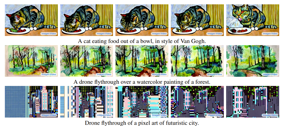
Fig 7: Snapshots of frames from videos generated by Imagen Video demonstrating the ability of the model to generate dynamics in different artistic styles. [2]
In this innovative training method, individual images are treated as single-frame videos. This is achieved by organizing standalone images into sequences that mimic the length of a video. The approach cleverly bypasses certain video-specific computations and attention mechanisms by employing masking techniques. This strategy enables the training of video models on extensive and diverse image-text datasets.
The outcome of joint training is the knowledge transfer from images to videos. Specifically, while training exclusively on natural video data allows the model to understand dynamics within natural environments, incorporating images into the training process enables it to learn about various image styles, including sketches, paintings, and more.
Sample results from Imagen Video
Prompt: A panda bear driving a car
Prompt: A teddy bear washing dishes
Experiments
We experimented with a video diffusion models using this diffusion model. We examine results when changing the number of inference steps below. All of the images use the same prompt, duration, and number of frames. The code we used to generate these samples is accessible in this Google colab notebook.
The prompt is ‘A futuristic cityscape at dusk, with flying cars weaving between neon-lit skyscrapers’.
We see from these results that a higher number of inference steps leads to an image that more accurately reflects the prompt. With 5 steps, the video hardly reflects the prompt. With 25 steps, a resemblance is shown but the image is largely warped and different from the desired result. With 50 steps, the image accurately shows the prompt.
Comparison
Imagen video generates much higher resolution videos compared to VDM. However, VDM has more flexibility in its usage since it allows for the generation of arbitrarily long videos via autoregression and the generation of videos conditioned on other videos.
Reference
[1] Ho, Jonathan, et al. “Video diffusion models.” arXiv:2204.03458 (2022).
[2] Ho, Jonathan, et al. “Imagen Video: High Definition Video Generation with Diffusion Models.” arXiv:2210.02303 (2022).
[3] Salimans, Tim, and Jonathan Ho. “Progressive Distillation for Fast Sampling of Diffusion Models.” In ICLR, 2022.
[4] Saharia, Chitwan, et al. “Image super-resolution via iterative refinement.” IEEE Transactions on Pattern Analysis and Machine Intelligence (2022).
[5] Brooks, Peebles, et al. “Video generation models as world simulators.” OpenAI (2024).
[6] Anonymous Authors. “Video Diffusion Models - A Survey.” Open Review, arXiv:2310.10647 (2023).