A Comparison of Point Cloud 3D Object Detection Methods
3D object detection is a very important task that is critical to many current and relevant problems. It has numerous applications for developing car technology involving features such as obstacle avoidance and autonomous driving. Another valuable application is medical imaging, specifically brain tumor segmentation. Our paper explores the most recent advances in 3D object detection using point clouds. Doing this, we acknowledge that work in this area is less progressed than with 2D object detection. We analyze performance and model design, evaluating prominent 3D object detection models VoxelNet, PointRCNN, SE-SSN, and GLENet with the widely used KITTI dataset as a common benchmark. In our examination, we determined that VoxelNet, as one of the earlier models in 3D object detection, had a poorer performance than the later advancements. After VoxelNet, PointRCNN performs next best, then SE-SSN, and then GLENet. With each development, we discuss how differences in design decisions and architecture contribute to improved average precision and inference times. These advancements in 3D object detection show a lot of promise and potential for future computer vision applications.
Intro
Background
3D Object Detection Task
3D object detection is a computer vision task in which objects are “detected” by generating 3D bounding boxes around the target objects. In particular, a 3D object detection model takes in an input which may consist of RGB images with depth, or 3D point clouds created by technology such as LiDAR (Light Detection and Ranging). The model will output a category label that signifies the classification of the object as well as a bounding box.
There are several applications to this task. One major area includes autonomous driving, as driverless cars need 3D object detection to provide the systems with information in order to predict vehicle paths. Another area includes housekeeping robots where a robot roams and cleans floors, needing to avoid crashing into objects as well as navigate around objects through object detection. Other examples include augmented or virtual reality, as well as medical imaging.
History
Throughout history, there have been several developments in 2D-object detection, however 3D-object detection using point clouds has been a new area of challenge as “LiDAR point clouds are sparse and have highly variable point density, due to factors such as non-uniform sampling of the 3D space, effective range of the sensors, occlusion, and the relative pose” (Voxelnet). In particular, classical approaches have been proposed including many that create their own feature representations manually. These approaches may project the point clouds to then obtain features, or they may break down the space into voxels, in which features are obtained from the voxels. These include examples like obtaining kernel features on depth images, using point signatures, and mapping patches to a sphere.
More recently, approaches use machine-learned features from a model. In 2017, PointNet was proposed which learns the features from the point clouds themselves. VoxelNet also proposes to use voxels in combination with a Region Proposal Network to learn the feature representation from a model. Some solutions use single as well as second stage detectors using region proposal features, and some methods also try to combine RGB images and point clouds to better learn features. One of the current best methods for the KITTI dataset is the SE-SSD which follows several models which “aim to exploit auxiliary tasks or further constraints … without introducing additional computational overhead during the inference” (SE-SSD). The current best model is GlenNet, which aims to decrease label uncertainty to improve upon existing models (GlenNet).
Evaluation Metrics
There are several evaluation metrics used in 3D object detection algorithms to gain an understanding of the model’s performance, the most common one being mean average precision (mAP). The mAP formula is based on a few submetrics: confusion matrix, intersection over union (IoU), precision and recall.
Confusion Matrix
A confusion matrix consists of four attributes:
- True positive (TP): the model correctly predicts a bounding box compared to the ground truth.
- True negative (TN): the model did not predict a bounding box that’s not part of the ground truth.
- False positive (FP): the model predicts a bounding box that’s not part of the ground truth.
- False negative (FN): the model did not predict a bounding box when there should be one in the ground truth.
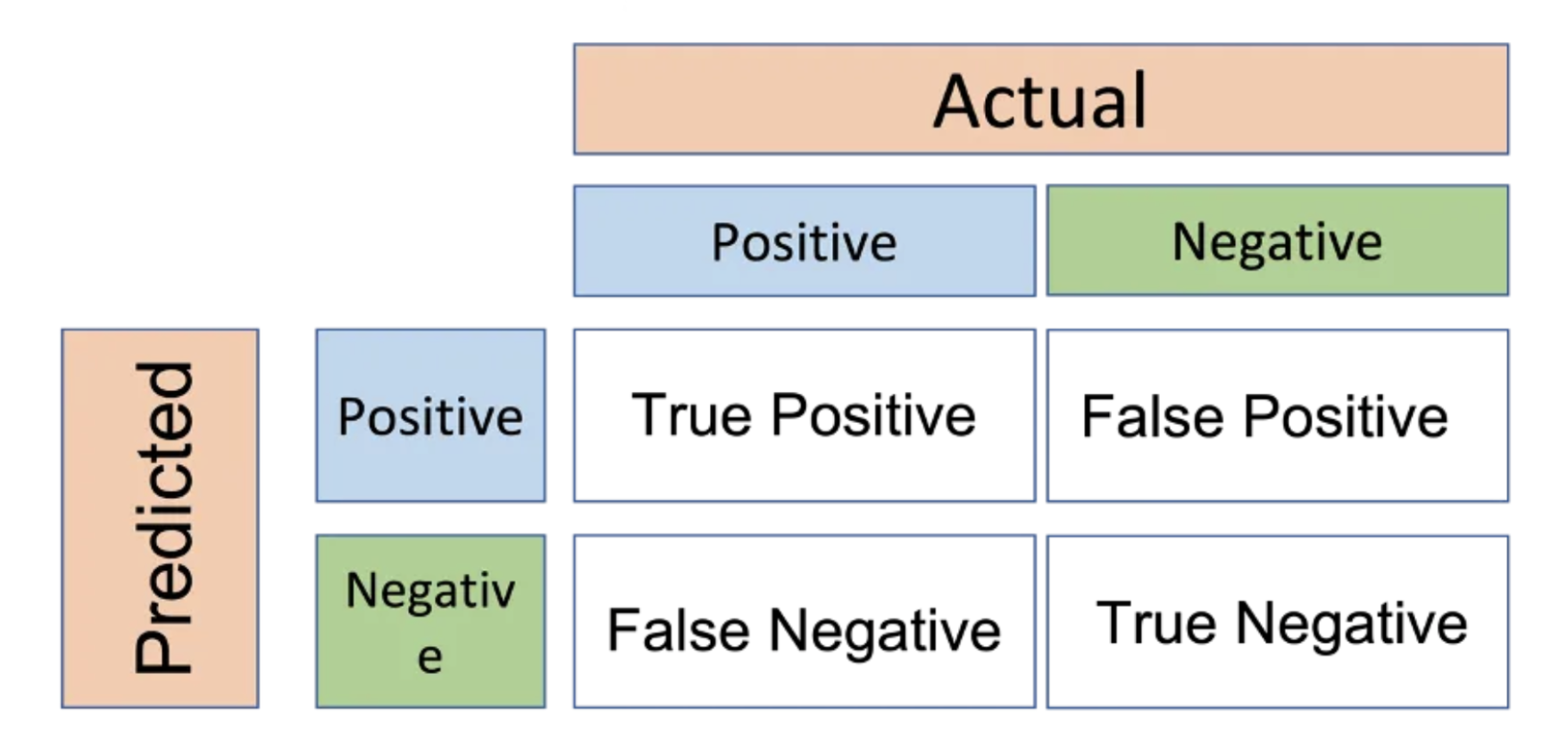
Fig 1. Confusion Matrix.
Intersection over Union (IoU)
IoU measures the overlap between the predicted bounding box and the ground truth bounding box. It is defined as the ratio between the area of intersection and the area of union of the two bounding boxes. If the predicted bounding box completely overlaps the ground truth bounding box, the IoU is 1. If the two bounding boxes do not overlap at all, the IoU is 0.
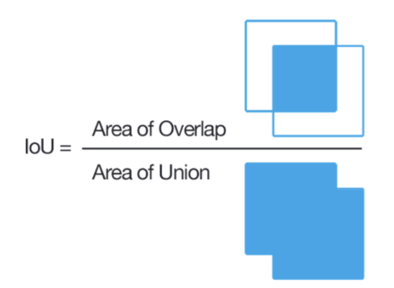
Fig 2. Intersection over Union.
In addition to IoU, a threshold value is needed to evaluate the performance of a 3D object detection model. This value denotes the minimum level of overlap between the predicted bounding box and the ground truth bounding box necessary for the model’s prediction to be deemed correct.
Precision
With the confusion matrix data, we can calculate precision which is a measure of how correct the model’s positive predictions are, which in the 3D object detection context would be the accuracy of the predicted bounding boxes. It is defined as the proportion of true positive predictions by the total number of positive predictions made.
\[Precision = \frac{TP}{TP + FP}\]Recall
We can also calculate the recall, which measures the model’s ability to identify all relevant objects of a class from a dataset (ground truths). It is defined as the ratio of true positives to the sum of true positives and false negatives.
\[Recall = \frac{TP}{TP + FN}\]Precision Recall Curve
The precision recall curve is a plot of the value of precision against recall for different confidence threshold values, a value obtained from the model for each prediction. This plot allows for visualization of which threshold yields the best results, which looks something like the image below.
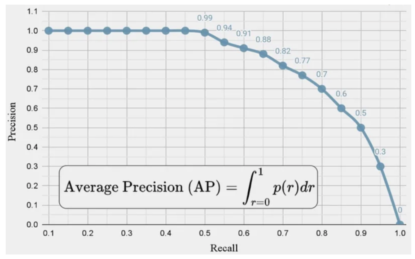
Fig 3. Precision Recall Curve.
Average Precision (AP)
The average precision can then be calculated after obtaining these submetrics. AP measures the precision of the object detection model at different recall levels. It can be calculated by taking the area under the precision recall curve. One AP value is calculated for each class in the dataset.
\[AP = \int_{r=0}^{1}{p(r)dr}\]Mean Average Precision (mAP)
Mean average precision is a metric that evaluates the trade-offs between precision and recall, providing a good measure for quantifying the performance of the model. After an AP value is calculated for each class, the mAP can be calculated by taking the average of the AP’s across all the classes.
\[mAP = \frac{1}{n}\sum_{i}^{n}{AP_i}\]Datasets
The KITTI dataset is one of the most commonly used benchmark datasets in 3D object detection tasks, particularly for autonomous driving. It is composed of six hours of traffic scenario recordings, which were recorded from a camera mounted on top of a car. It is a diverse dataset that includes a variety of real-world scenarios which vary from urban to rural driving conditions, freeway to local traffic, and static to dynamic objects. The KITTI 3D object detection dataset consists of 3713 training images, 3769 validation images, and 7518 testing images. This data set includes 3D annotated ground-truth bounding boxes which are labeled ‘Car’, ‘Pedestrian’, and ‘Cyclist’. The dataset is divided into ‘Easy’, ‘Medium’, and ‘Hard’ categories based on bounding box size, level of occlusion, and truncation percentages.
Models
VoxelNet
As opposed to traditional methods, VoxelNet incorporates the Region Proposal Network, which had been at the time successful for non point cloud detection tasks, with feature learning to detect objects in the 3D LiDAR point cloud space. It is an end-to-end model that is trainable with benefits of efficiency and feature representation from its sparse point structure and parallel voxel grid processing.
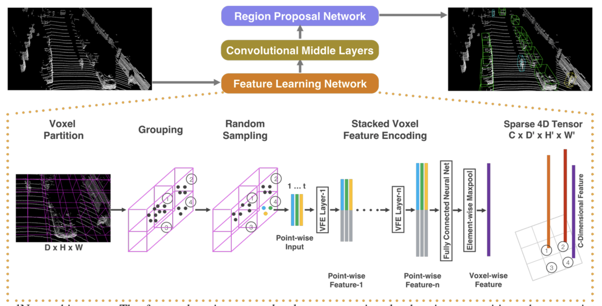
Figure 4. Architecture, with focus on the feature learning network. [4].
The architecture of the model consists of three main stages: feature learning network, convolutional middle layers, and region proposal network. The 3D point space is fed into the feature learning network which provides an encoding for the space, this encoding is fed into the convolutional middle layers, and then the region proposal network to generate final decisions. This model introduced a novel Voxel Feature Encoding Layer (VFE), which encodes voxels into high dimensional feature representations and allows for point and point interactions through its feature development. In particular, the feature learning network divides the 3D space into voxels, groups these voxels, and randomly samples T points to saves computation and mitigate imbalances. Subsequently, the VFE layer transforms the input by augmenting each point by its offset to the centroid. This input is passed into a fully connected layer to retrieve the point-wise features, which is augmented with the local aggregated feature to obtain an encoding. A sparse vector representation for nonempty voxels was used to save memory and computation.
The output 4D tensor from the feature learning network is next fed into convolutional middle layers and then the Region Proposal Network (RPN) which then maps the output to a probability score map and regression map, which form the basis of object detection. The architecture of the RPN consists of three blocks of fully connected layers.
Overall, the model was trained on the GPU efficiently, and used the KITTI 3D object detection benchmark as a task to detect cars, pedestrians, and cyclists. An input buffer on the GPU was created, and the VFE only utilized GPU parallelizable operations. The dense voxel grid used in the convolutional middle layers and the final RPN were both trainable on the GPU. The loss function that was minimized included a combination of normalized classification loss for positive and negative anchor points with binary cross entropy loss, as well as an additional regression loss. The model was evaluated on Car, Pedestrian/Cyclist areas at different difficulty levels. Results showed that the model performed better than the hand-crafted feature model in most areas.
In general, the benefits of this model include its machine learned features, and efficient implementation by utilizing the GPU to do parallel voxel grid operations, as well as by using sparse vector representations. Disadvantage is that this model needs to be extended to image 3D-object detection, joint LiDAR, and can further improve in localization accuracy and detection results. [4]
PointRCNN
PointRCNN utilizes a raw point cloud to generate a bounding box for 3D object detection. It is composed of two core stages and is the first two-stage 3D object detector.
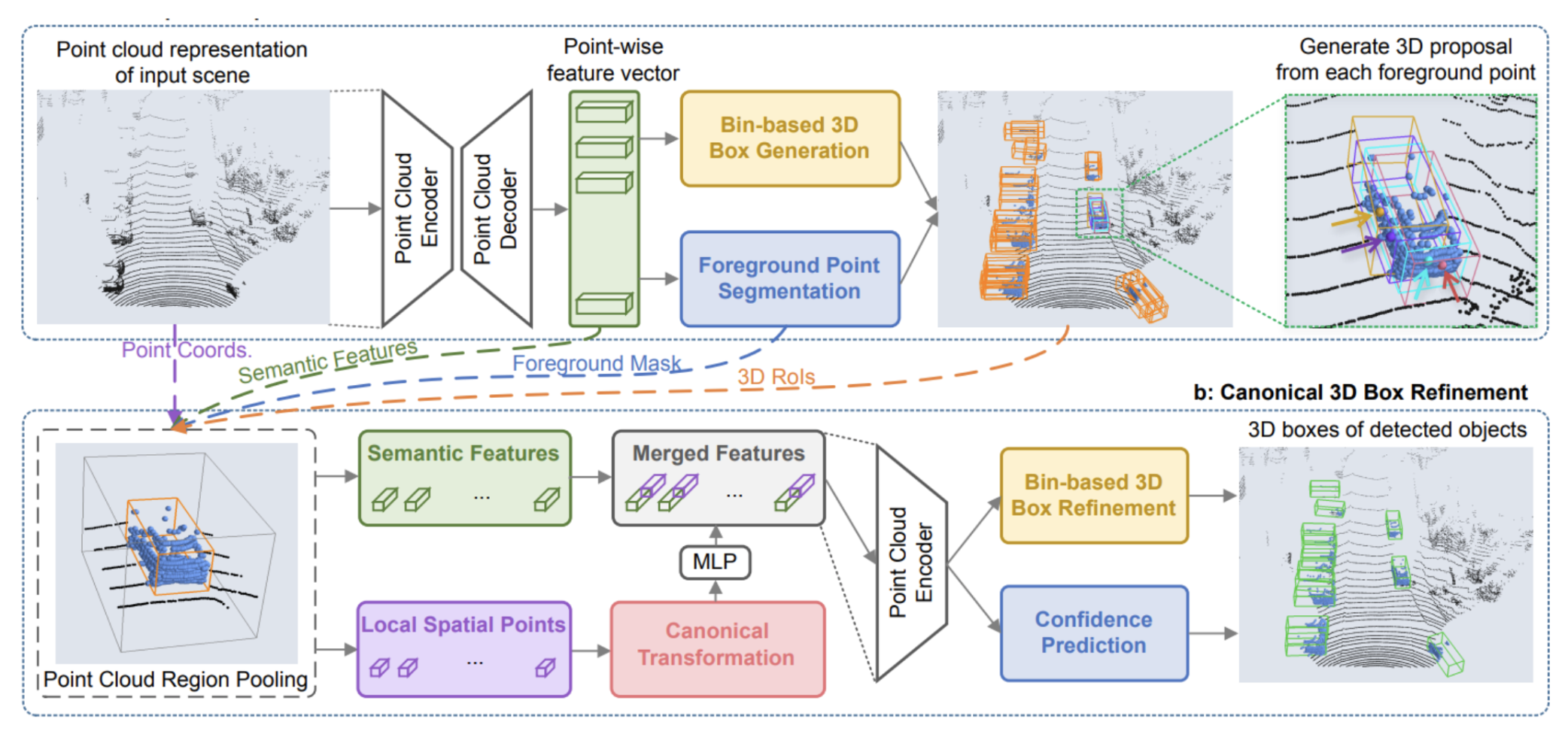
Figure 6. PointRCNN architecture. [1].
The first stage is allocated for the 3D proposal generation and is based on whole-scene point cloud segmentation. This method relies on the observation that 3D scenes are naturally separated and thus 3D object segmentation masks can be obtained by their bounding box. In this stage, the model generates a few high-quality 3D proposals from the point cloud using a bottom-up approach. It does this by using learned point-wise features to segment the raw point cloud and then generate 3D proposals. The 3D boxes for these proposals are generated through a bin-based 3D bounding box approach. A key component of this approach is also foreground segmentation which ensures that the model gets contextual information for precision-making. This approach for stage 1 is more efficient than other models. The model’s proposal only includes a small number of high-quality proposals. Consequently, it avoids the complexities that come with a large set of 3D boxes in the 3D space.
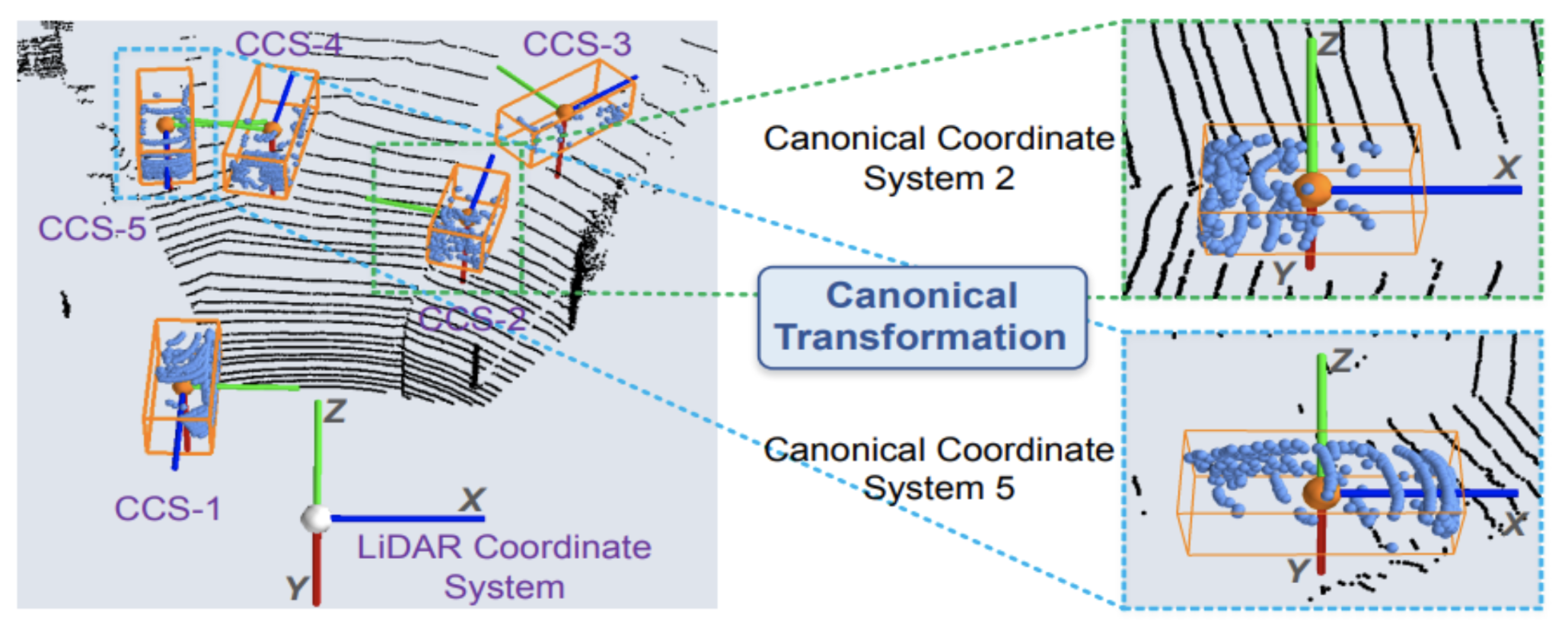
Figure 6. Canonical Transformation. [1].
The second stage involves refining the 3D bounding box proposals, specifically the locations and orientations. The points undergo a canonical transformation to a Canonical Coordinate System, CCS, demonstrated in Figure 6. Then the model works on refining the boundary based on previously generated box proposals. It looks at semantic and local spatial features combined. In this stage, the model considers the points individually, refining them if they are within a pre-defined expanded bounding box.
This two-stage bottoms-up approach using a raw point cloud performs extremely well on the KITTI dataset. It performs well for the 3D object detection problem on the KITTI dataset and has a high recall. It is also computationally efficient while outperforming other models. [1]
Self-Ensembling Single Stage object Detector (SE-SSD)
Unlike PointRCNN, the SE-SSD model, developed by Zheng et al, is designed as a single-stage detector for its simpler structure and based only on LiDAR point clouds. This fully supervised model consists of a teacher SSD and a student SSD, where the teacher SSD produces a bounding box and confidence as the student’s soft targets. Then there is a formulated consistency constraint based on IoU matching that filters soft targets and pairs them with the student predictions, which should produce a consistency loss to reduce misalignment between the target and prediction. SE-SSD also uses hard targets as the final targets for the model convergence, where the model uses orientation-aware distance-IoU (ODIoU) loss to supervise the student with constraints on the center and orientation of the predicted bounding box. Additionally, SE-SSD implements a new shape-aware augmentation scheme on top of the conventional one to encourage the model to infer the object shape from incomplete information. The architecture of this model is shown below in Figure 7.
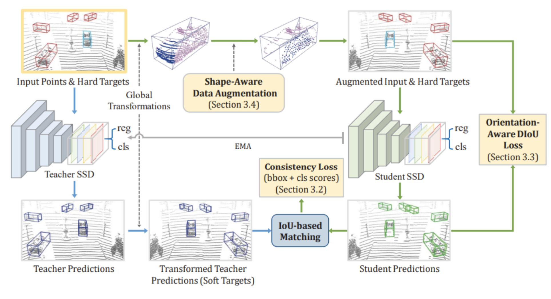
Figure 7. Architecture of the SE-SSD model. [3].
The teacher and student SSD are initialized with a pre-trained SSD model and trained simultaneously. The blue path shown in Figure 7 is where the teacher SSD produces predictions from the raw input and a set of transformations are applied to them. They are then passed as soft targets to supervise the student SSD. The green path in Figure 7 is where the same input undergoes the same set of transformations as the blue path and then goes through the shape-aware data augmentation (labeled as Section 3.4 in the figure). This augmented input is taken to the student SSD and trained with consistency loss (labeled as Section 3.2 in the figure). The augmented input along with the hard targets are used to supervise the student with the ODIoU loss (labeled as Section 3.3 in the figure).
Overall, at each iteration during training, the student SSD is optimized with the consistency and ODIoU loss, and the teacher is updated using only the student parameters, obtaining knowledge from the student to produce more soft targets to supervise. The advantages of SE-SSD include a simpler architecture that requires fewer computational resources since it is a single-stage object detector rather than a two-stage object detector. It is also better at generalization and the results achieve state-of-the-art performance in accuracy and efficiency for object detection from point clouds. However, there are some disadvantages including the complexity of the self-ensembling technique which may lead to longer training times. SE-SSD also requires additional hyperparameters and is sensitive to erroneous predictions during the training process. [3]
GLENet
GLENet, developed by Zhang et al, aims to address the uncertain and complex nature of 3D object ground-truth annotations through a probabilistic approach as opposed to a deterministic one. Traditional 3D object detection architectures take a deterministic approach and face challenges in situations involving occluded objects, incomplete LiDAR data, or subjective data labeling errors. GLENet on the other hand is a generative deep learning framework derived from conditional variational autoencoders that improves upon the robustness of object detectors by introducing label uncertainty.
GLENet accounts for variation in bounding boxes by mapping point clouds to multiple potential ground truth bounding boxes. The label uncertainty of each object is generated based on the variance of the distribution of its potential ground-truth bounding boxes. As seen in Figure 8, GLENet predicts a range of bounding boxes for each 3D point cloud. For incomplete point clouds with 1 or 5 points, there is higher variance in the bounding boxes and thus a higher label uncertainty. For more complete point clouds with 335 or 693 points, there is lower variance and more consistent bounding boxes, resulting in a lower label uncertainty.
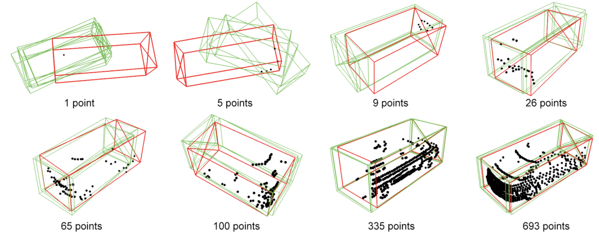
Figure 8. Bounding boxes generated by GLENet on the KITTI dataset in green, ground truth annotations in red, and point cloud in black. [2].
Conditional variational autoencoders (CVAE) are used in this context to generate the distribution of bounding boxes, modeled as a Gaussian distribution. Each distribution is conditioned on a point cloud, and the conditional distribution is generated based on equation .., where C is the point cloud, 8 is the ground truth bounding box of the point cloud C, and z is an intermediate variable. The variance of the distribution can be estimated from random samples of the bounding box distribution using the Monte Carlo technique.
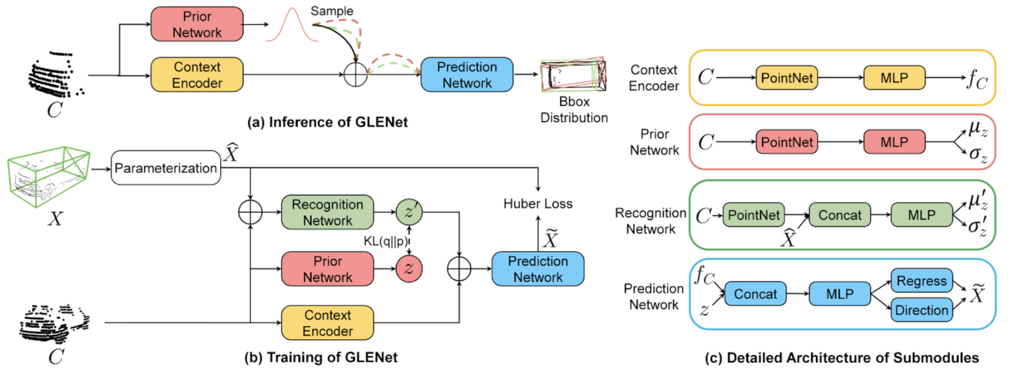
Figure 9. The training and inference worklflows of GLENet [2].
As seen in Figure 9, the architecture of GLENet can be split into the inference process and the training process. During the inference process, a point cloud C is taken in as the input, and the sampling process is performed to output a variety of plausible bounding boxes. The input is first passed into the prior network, which consists of PointNet and MLP layers, to predict the mean and standard deviation of the Gaussian distribution. Context information outputted from the context encoder is then concatenated with multiple samples of the distribution and passed into a prediction network. The prediction network takes the concatenated inputs and passes them through MLP layers to predict the shape and size, position, and orientation of bounding boxes for each sample. Furthermore, during the training process, a point cloud C and its corresponding bounding box X are taken in as inputs. The bounding box is parameterized and concatenated with the point cloud and passed through the recognition network. Then, a combination of the context encoder, prior network, and prediction network are used to optimize parameters used for estimating the Gaussian distribution. The loss function is a combination of Huber loss, binary cross-entropy loss, and KL-divergence.
GLENet is integrated with existing 3D object detectors to transform deterministic models into probabilistic models by representing the detection head and ground-truth bounding boxes with probability distributions. The model was integrated with the Voxel R-CNN framework and evaluated on the KITTI test set, which proved to greatly surpass most state-of-the-art detection methods in performance. It has been shown to significantly increase the localization reliability and detection accuracy of models, which is desirable for real-world applications. However, while GLENet is a powerful framework, some drawbacks include high complexity and computational costs, the lack of true distribution information, and the limited ability to generalize to more extensive datasets. [2]
Implementation: VoxelNet
We decided to implement VoxelNet using the KITTI dataset. We started by downloading the KITTI dataset’s Velodyne point clouds, training labels, camera calibration information, and left color images. When training we divided the 3D point cloud space into equally spaced voxels. Then we used random sampling to determine which sections to sample. This helps to save computationally and reduce point imbalance. Then we augmented the selected points before training. The fully connected neural network consists of a linear layer, batch normalization, and ReLu layer. Through element-wise max pooling we determine the locally aggregated features. This is aggregated with the point-wise features. We use the convolutional middle layers to transform the voxels into dense 4D feature maps and shrink the feature map to a fourth of its size. These layers are brought together in a region proposal network with 3 blocks of layers, giving us our final detection results.[5]
class VFELayer(object):
    def __init__(self, out_channels, name):
        super(VFELayer, self).__init__()
        self.units = int(out_channels / 2)
        with tf.variable_scope(name, reuse=tf.AUTO_REUSE) as scope:
            self.dense = tf.layers.Dense(
                self.units, tf.nn.relu, name='dense', _reuse=tf.AUTO_REUSE, _scope=scope)
            self.batch_norm = tf.layers.BatchNormalization(
                name='batch_norm', fused=True, _reuse=tf.AUTO_REUSE, _scope=scope)
    def apply(self, inputs, mask, training):
        pointwise = self.batch_norm.apply(self.dense.apply(inputs), training)
        aggregated = tf.reduce_max(pointwise, axis=1, keep_dims=True)
        repeated = tf.tile(aggregated, [1, cfg.VOXEL_POINT_COUNT, 1])
        concatenated = tf.concat([pointwise, repeated], axis=2)
        mask = tf.tile(mask, [1, 1, 2 * self.units])
        concatenated = tf.multiply(concatenated, tf.cast(mask, tf.float32))
        return concatenated

class ConvMiddleLayer(tf.keras.layers.Layer):
    def __init__(self, out_shape):
      super(ConvMiddleLayer, self).__init__()
      self.out_shape = out_shape
      self.conv1 = tf.keras.layers.Conv3D(64, (3,3,3), (2,1,1), data_format="channels_first", padding="VALID")
      self.conv2 = tf.keras.layers.Conv3D(64, (3,3,3), (1,1,1), data_format="channels_first", padding="VALID")
      self.conv3 = tf.keras.layers.Conv3D(64, (3,3,3), (2,1,1), data_format="channels_first", padding="VALID")
      self.bn1 = tf.keras.layers.BatchNormalization(trainable=True)
      self.bn2 = tf.keras.layers.BatchNormalization(trainable=True)
      self.bn3 = tf.keras.layers.BatchNormalization(trainable=True)
    def call(self, input):
      out = tf.pad(input, [(0,0)]*2 + [(1,1)]*3)
      out = tf.nn.relu(self.bn1(self.conv1(out)))

      out = tf.pad(out, [(0,0)]*3 + [(1,1)]*2)
      out = tf.nn.relu(self.bn2(self.conv2(out)))

      out = tf.pad(out, [(0,0)]*2 + [(1,1)]*3)
      out = tf.nn.relu(self.bn3(self.conv3(out)))
      return tf.reshape(out, self.out_shape)
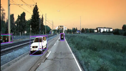
Figure 10. VoxelNet Object Detection Result.[5].
Results/Comparison
The models discussed above were evaluated on the KITTI server and compared against the 3D and BEV average precision benchmarks with an IoU threshold of 0.7. They were conducted on the car category of this dataset with three difficulty levels in the evaluation: easy, medium, and hard. We compare the results of these models upon the KITTI Cars Easy dataset below. Results are obtained from the respective journal articles.
| Method | Easy | Mod | Hard | mAP |
|---|---|---|---|---|
| VoxelNet [4] | 77.82 | 64.17 | 57.51 | 66.5 |
| PointRCNN [1] | 86.96 | 75.42 | 70.70 | 77.77 |
| SE-SSD [3] | 91.49 | 82.54 | 77.15 | 83.73 |
| GLENet-VR [2] | 91.67 | 83.23 | 78.43 | 84.44 |
The VoxelNet model performed well with a mAP of 66.5%. This was based on average precisions of 77.82%, 64.17%, and 57.51% for easy, medium, and hard difficulty levels respectively. VoxelNet was the first model of its kind that used point cloud-based 3D detection. It was very different from traditional techniques and marked progress in the 3D object detection space. Newer models like PointRCNN, however, outperform VoxelNet. PointRCNN has a mAP of 77.77% and average precisions of 86.96%, 75.42%, and 70.70% for the same categories. PointRCNN is a two-stage point cloud-based model, while VoxelNet is a one-stage end-to-end trainable model. Point RCNN takes a more refined approach with its two stages. In its first stage it generates bounding box proposals. In the second stage, it refinines them and implements region-based feature extraction. Furthermore, since PointRCNN operates directly on point clouds, it avoids the information loss that voxel encoding introduces. These differences allow Point-RCNN to capture more details and work with more irregularities, resulting in higher precision and better overall performance.
In terms of 3D AP, SE-SSD consistently outperforms PointRCNN, achieving an AP of 91.49%, 82.54%, 77.15% for easy, medium, and hard difficulty levels respectively with a mAP of 83.73%. On the other hand, PointRCNN yields slightly lower results with AP scores of 86.96%, 75.42%, and 70.70% with a mAP of 77.77%. Furthermore, SE-SSD demonstrates faster inference with an inference time of 30.56ms while PointRCNN achieved an inference time of 100ms. The differences in performance can be attributed to several factors, including architectural design, methodology, and computational complexity. PointRCNN is built upon a two-stage region-based framework, where it generates region proposals followed by region-wise feature extraction and classification. This two-stage architecture contributes to PointRCNN’s slower inference time compared to SE-SSD’s inference time as it relies on more complex processing steps and refinement. SE-SSD on the other hand is a single-stage object detector which requires fewer computational resources and eliminates the need for having to generate region proposals. Its architecture focuses primarily on predicting the bounding boxes and probabilities, allowing for more efficient processing of input data to results, which contributes to its faster inference speed than PointRCNN. Although the results from PointRCNN are slightly lower than SE-SSD’s, it still has its advantages. PointRCNN’s two-stage architecture and refinement process makes it more adept at accurately localizing objects in dense point clouds and complex environments. However, this enhanced accuracy comes at the expense of increased computational resources.
GLENet was integrated with the Voxel R-CNN framework to create the probabilistic 3D object detector, GLENet-VR. GLENet-VR performs exceptionally well on the KITTI test set and is currently ranked number one among all published LiDAR-based 3D object detection approaches. It achieved an average precision of 91.67% on the easy dataset, 83.23% on the medium dataset, and 79.14% on the hard dataset. When comparing GLENet-VR to VoxelNet, PointRCNN, and SE-SSD, we observe that it outperforms all models on the easy, medium, and hard datasets. GLEN-VR is able to perform better than other models due to its addition of probabilistic modeling to measure 3D label uncertainty. Combining it other state-of-the-art detectors enhances the robustness, reliability, and detection accuracy of these models. When GLENet is integrated with stronger base 3D detection models, it is naturally able to achieve more accurate detection results. Its use of conditional variational autoencoders to generate bounding box distributions has shown to generate fewer false positive bounding boxes and accurately capture more occluded or distant objects. However, GLENet-VR uses Voxel R-CNN as the base detector, and its performance is dependent on the performance of the base detector. Since Voxel R-CNN does not have the best overall performance among other base detection models, it is possible that GLENet could achieve even better performance in the future if integrated with an even more robust model.
Conclusion
There has been significant progress made in the field of 3D object detection throughout the years. Through our comparisons of state-of-the-art 3D object detection models, we observe how the architecture and design decisions of detection models have transformed over time. Advancements from VoxelNet to PointRCNN, SE-SSD, and finally GLENet, have significantly enhanced the robustness and performance of 3D object detection tasks. The field continues to evolve and address challenges with computational resources, generalization to new scenarios, and robustness to environmental variability. These ongoing efforts strive to develop models that can capture the full complexities of 3D object detection tasks.
Reference
[1] Shi, S., Wang, X., & Li, H. (2018, December 11). PointRCNN: 3D object proposal generation and detection from point cloud. arXiv.Org. https://arxiv.org/abs/1812.04244
[2] Zhang, Y., Zhang, Q., Zhu, Z., Hou, J., & Yuan, Y. (2022, July 6). GLENet: Boosting 3D object detectors with generative label uncertainty estimation. arXiv.Org. https://arxiv.org/abs/2207.02466
[3] Zheng, W., Tang, W., Jiang, L., & Fu, C.-W. (2021, April 20). SE-SSD: Self-Ensembling single-stage object detector from point cloud. arXiv.Org. https://arxiv.org/abs/2104.09804
[4] Zhou, Y., & Tuzel, O. (2017, November 17). VoxelNet: End-to-End learning for point cloud based 3D object detection. arXiv.Org. https://arxiv.org/abs/1711.06396
[5] Adusumilli, G. (2020, September 18). Lidar Point-cloud based 3D object detection implementation with colab. Medium. https://medium.com/towards-data-science/lidar-point-cloud-based-3d-object-detection-implementation-with-colab-part-1-of-2-e3999ea8fdd4