Visuomotor Policy Learning
In visuomotor policy learning, an agent learns to excel at a sequential decision-making task involving visual inputs and motor control. Two important applications include autonomous driving and robotics control.
- Introduction
- Approaches to Visuomotor Policy Learning
- Policy Pretraining
- A Deep Dive into UniAD [6]
- References
Introduction
In visuomotor policy learning, an agent learns to excel at a sequential decision-making task involving visual inputs and motor control. In this report, we explore applications in autonomous driving and robotics control with imitation learning (IL) and reinforcement learning (RL) approaches, with more focus on autonomous driving and imitation learning.
Problem Formulation
Policy learning is often formulated as some form of a Markov Decision Process (MDP) from Reinforcement Learning, where the agent’s policy’s choice of action depends only on the current state.
Our goal is to learn a policy \(\pi_{\theta}(a_t \mid o_t)\) that determines the agent’s action based on its observation of its environment. The policy output can be binary (deterministic policy), or probabilities (stochastic policy).
At each time step, the agent:
-
Observes the current state \(s_t\) to generate observation \(o_t\).
-
Chooses an action based on its policy \(\pi_{\theta}(a_t \mid o_t)\)
-
Receives reward \(R_t\) (or loss \(L_t\))
A training trajectory is such a sampled sequence of states, actions, and (optionally) rewards, given by \(\tau = \{o_1, a_1, r_1, \dots, o_T, a_T, r_T\}\).
Then, the objective is to maximize the expected reward: \(\max_{\theta} E_{\tau \sim \pi_{\theta}}[\sum_{t=1}^T \gamma^t r_t]\), with discount factor \(\gamma\), or minimize the expected loss: \(\min_{\theta} E_{\tau \sim \pi_{\theta}}[\sum_{t=1}^T L_t(o_t, a_t)]\).
Approaches to Visuomotor Policy Learning
For policy learning in general, there are two main approaches: imitation learning and reinforcement learning.
Imitation learning is a supervised approach where the agent learns based on expert demonstrations (e.g. human behavior). For instance, collecting human driving data and training an agent to take the same actions as the human driver is an example of imitation learning known as behavior cloning.
Reinforcement learning learns by exploring different states/actions, deciding whether these states/actions are good based on reward feedback, and optimizing its value function and/or policy.
The choice between the two approaches comes down to use case. Imitation learning has good stability but performs poorly when encountering distributional shift (observed data distribution is significantly different from demonstration data distribution), often cannot recover from errors, and can only become as good as the demonstrations. Reinforcement Learning is more unstable, has to address exploration-exploitation tradeoff, requires a well-defined reward function, but can achieve superhuman-level performance.
For example, in autonomous driving, imitation learning is preferred since ways to perform an action (e.g. turn left) are more unimodal, exploration is less important, and complex scenarios are difficult to handle for both IL and RL. In robotics control, IL and RL are both applicable. In playing video games, RL has a significant advantage over IL in being able to achieve superhuman-level performance.
Policy Pretraining
Regardless of the chosen approach, sampling data from the environment is expensive. Therefore, as with many tasks facing data scarcity, most implementations pretrain the vision encoder of the model in some way. Here we discuss three approaches, taken from [5], [1], [6], [3].
Approach 1: Decoupled vision policy pretraining [5]
In “End-to-End Training of Deep Visuomotor Policies” (2016) [5], Levine et al. uses the following visuomotor policy architecture:

Fig 1. Visuomotor policy architecture from Levine et al. [5].
Levine et al. initializes a vision encoder (with first-layer weights from ImageNet pretraining) and pretrains the vision encoder to predict elements of the world state not given in the observations (e.g. positions of objects in the scene).
They also pretrain a “cheating” teacher policy using reinforcement learning that learns actions given full world-state information, which is later used as an imitation learning guidance signal for the observation-based policy.
Then, they optimize their model using guided policy search with BADMM as their optimization algorithm (a convex optimization algorithm, hence the presence of Lagrange multipliers), whose objective contains both a RL (trajectory) loss and an imitation learning (divergence penalty) loss:

Fig 2. Loss function used by Levine et al. [5].
Overall, the main disadvantage of this pretraining approach is that it requires knowing the full world state, which makes data collection more difficult.
Approach 2: Contrastive Pretraining [1]
In “Learning to Drive by Watching YouTube Videos: Action-Conditioned Contrastive Policy Pretraining” [1], Zhang et al. modify MoCo [2], a general contrastive learning approach and apply it to visuomotor policy tasks.
Specifically, in addition to the instance contrastive pair (ICP) used by MoCo, they introduce Action Contrastive Pairs (ACP), where if two images are labeled with similar actions (e.g. turning 35 degrees left & turning 40 degrees left), they are considered positive pairs, regardless of the content of the image.
Since YouTube videos do not have actions labeled, Zhang et al. had to additionally learn an inverse dynamics model using the NuScenes dataset and apply it on the YouTube videos to generate pseudo action labels.
Below is their training pipeline:
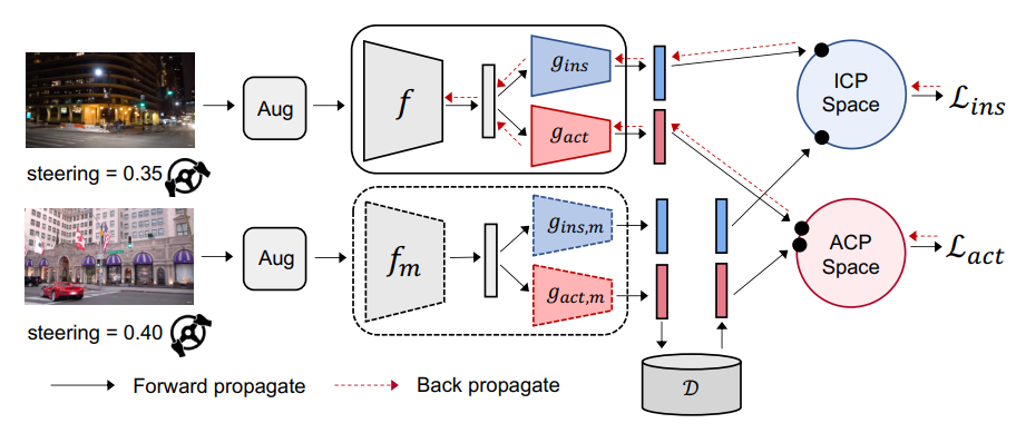
Fig 3. ACO Architecture from Zhang et al. [1].
They train encoder \(f\) and projectors \(g_{ins}\), \(g_{act}\) (where \(f_m\), \(g_{ins,m}\), \(g_{act,m}\) are momentum-smoothed versions of \(f\), \(g_{ins}\), \(g_{act}\) respectively) to optimize the joint ICP and ACP loss \(\lambda_{ins} \mathcal{L}_{ins}+\lambda_{act} \mathcal{L}_{act}\), where \(\mathcal{L} = -\log \frac{\sum_{z^+ \in P(z^q)} \exp(z^q \cdot z^+ / \tau)}{\sum_{z^- \in N(z^q)} \exp(z^q \cdot z^- / \tau)}\).
For ICP, positive pairs include only the image itself. For ACP, positive pairs include all images with similar-enough actions, specifically \(P_{act}(z^q) = \{z \mid \lVert \hat{a} - \hat{a}^q \rVert < \epsilon, (z, \hat{a}) \in K\}\), where \(K\) is the key set (the subset of images we’re currently comparing to).
Empirically, they demonstrate significant improvement over MoCo:

Fig 4. Results from Zhang et al. [1].
Approach 3: Auxiliary Tasks Pretraining [6]
In “Planning-oriented Autonomous Driving”, Hu et al. use a frozen pretrained BEVFormer [10] and pretrain their model on auxiliary vision tasks: object tracking and panoptic segmentation. In the pipeline below, they pretrain up to the perception stage, before continuing training on all tasks.

Fig 5. UniAD pipeline [6].
Approach 4: Adapting Large Pretrained Models
In “DriveLM: Driving with Graph Visual Question Answering”, Sima et al. explores using vision-language models (VLM) to do autonomous driving.
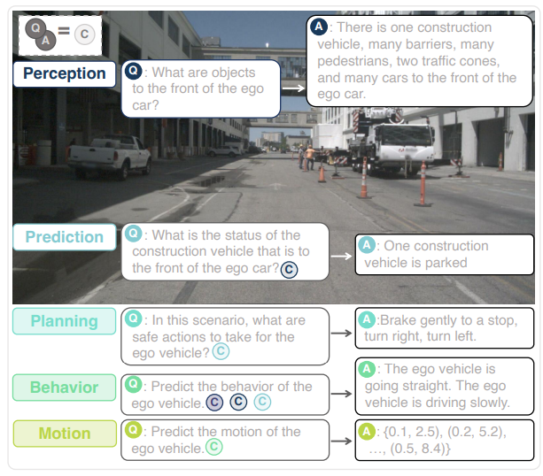
Fig 6. DriveLM-Agent inference examples from Sima et al. [3].
For their DriveLM-Agent baseline, they chose BLIP-2 [9] as their base model, which comes with robust vision language reasoning.
Main advantages include robust generalization and interpretable step-by-step reasoning, but some downsides include currently inferring only based on the current video frame, significantly slower inference speed (10x slower than single-frame UniAD), and unnaturalness in discretizing and tokenizing a continuous trajectory (see page 24 of [3] for more details).
A similar paper “RT-2: Vision-Language-Action Models Transfer Web Knowledge to Robotic Control” [4] was also released a few months prior to DriveLM for robotics control, which takes a similar line of thought.
A Deep Dive into UniAD [6]
Now let’s take a deep dive into one SOTA visuomotor policy architecture, and analyze it component by component. We chose UniAD [6], since it is a significant improvement over previous methods (including LiDAR-based approaches) and contains a lot of engineering tricks worth taking a look at.
UniAD adopts a joint trajectory loss and imitation learning approach (similar to [5]), but trains everything with supervision (no reinforcement learning).
From the pipeline below, UniAD contains 6 components:
- Backbone
- TrackFormer (object tracking task)
- MapFormer (panoptic segmentation task)
- MotionFormer (trajectory prediction task)
- OccFormer (occupancy prediction task)
- Planner (planning task)
Backbone
The backbone used in UniAD is a frozen BEVFormer [10], which modifies the original transformer architecture by adding temporal self-attention and spatial cross-attention (sparse attention mechanisms based on Deformable Attention [8]). Additionally, it adopts an RNN-style temporal component, where historical BEVFormer features are passed between adjacent time steps sequentially.
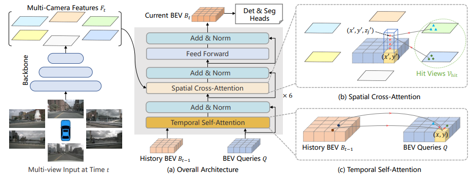
Fig 7. BEVFormer Architecture [10].
Deformable Attention
Deformable attention is a sparse attention mechanism that does local offset sampling rather than querying the whole space.
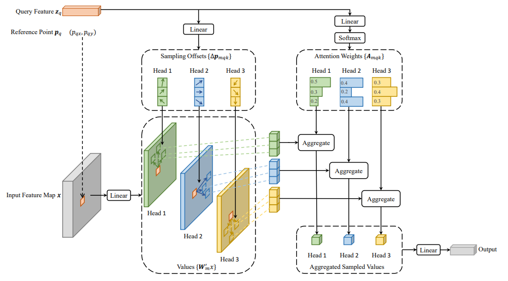
Fig 8. Deformable Attention Visualization [8].
As a formula, Deformable Attention is written as \(\text{DeformAttn}(z_q, p_q, x) = \sum_{m=1}^M W_m [ \sum_{k=1}^K A_{mqk} \cdot W_m' x(p_q + \Delta p_{mqk}) ]\), where \(M\) denotes number of heads, \(K\) denotes number of sampled keys with \(K \ll HW\), the size of the image.
Temporal Self-Attention and Spatial Cross-Attention
Spatial cross-attention (SCA) can be interpreted as sampling over the \(i\)th camera’s feature map \(F_t^i\) via projections of reference points (\(P(p, i, j)\), the projected location of the \(j\)th reference point for query \(Q_p\)). Formally, it is given by:

Fig 9. SCA Equation from BEVFormer. [10].
Temporal self-attention (TSA) queries over itself and features from the previous BEVFormer time step (recall the RNN-like feature passing) from the current query position \(p = (x,y)\) on the grid, given by:

Fig 10. TSA Equation from BEVFormer. [10].
For more details, check out the original paper [10].
TrackFormer
Fig 11. Object detection and tracking with TrackFormer. Video generated on GCP based on [6].
TrackFormer follows the BEVFormer [10] design, taking the MOTR [11] approach, where object detection is done similar to DETR [12], but on each subsequent frame, detected objects from previous frames are fed back in to act as tracking queries, until the model no longer detects the object with high confidence. This idea is visualized in the figure below:

Fig 12. MOTR Visualization [11].
MapFormer
MapFormer [6] is from Panoptic SegFormer [7], which modifies DETR to do panoptic segmentation based on attention masks. Specifically, they added a mask decoder that attends over the encoded features using queries from the location decoder / transformer encoder and supervises the attention map to predict the corresponding mask.
An output mask is computed at every layer during training for better supervision, but at inference time, only the last mask is taken as output.

Fig 13. Panoptic SegFormer architecture [7].
For more implementation details, please consult the original paper [7].
MotionFormer
Fig 14. Trajectory Prediction with MotionFormer. Video generated on GCP based on [6].
MotionFormer predicts agents’ future trajectories by modeling interactions between the agent to predict and three other entities: other agents (from TrackFormer), things (from MapFormer), and goal point (BEV features from backbone).
The authors take special care to encode as much positional information about the agent as possible.
Specifically:
-
\(I_s\) denotes the scene-level anchor, which represents prior movement statistics in world coordinates (it is the agent anchor but rotated and translated to world coordinates based on location and heading angle),
-
\(I_a\) represents the agent-level anchor, which is same thing as \(I_s\) but in local coordinates.
-
\(\hat{x}_0\) is the agent’s current position
-
\(\hat{x}_T^{l-1}\) is the agent’s predicted endpoint from previous layer. The intention is to gradually refine the prediction as the layers get deeper.
In training, both \(I_s\), \(I_a\) are based on ground-truth trajectories to avoid accumulating error.
After adding the query position onto the query context, they are fed through cross-attention modules, where standard attention is used for agent and map queries, while sparse attention is used for goal point query.
Note that everything is computed for \(K\) different modalities (to support multimodal trajectory distributions, e.g. turn left vs turn right vs continuing straight at an intersection).
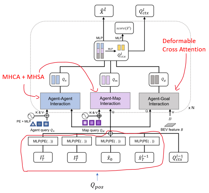
Fig 15. MotionFormer architecture [6], with annotations by me.
OccFormer
OccFormer predicts agents’ future occupancy in an RNN-style. At each layer, OccFormer takes in \(F\) (BEV features), \(Q_A\) (agent track query), \(P_A\) (agent position), and \(Q_X\) (motion query, max-pooled over the \(K\) modalities predicted in MotionFormer).
According to the authors, a cross-attention mask based on agent and scene features is computed to enhance location alignment between agents and pixel. The mask-features computed from agent is also reused in decoder for occupancy prediction with similar intuitive reason.
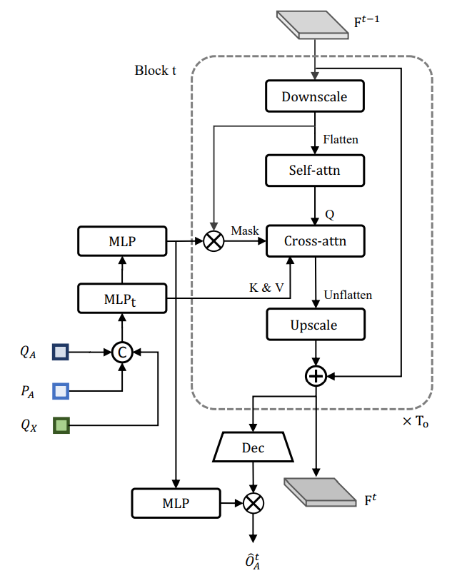
Fig 16. OccFormer architecture. [6]
Planner
Fig 17. Planning with Planner. Video generated on GCP based on [6].
Similar to OccFormer, planner takes in BEV features and agent features from TrackFormer and MotionFormer. However, here the max pooling happens after the command is processed, which selects the modality desired.
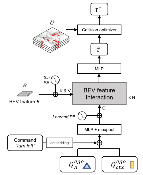
Fig 18. Planner architecture. [6]
The authors further avoids collisions by adding a collision avoidance loss onto the regular imitiation loss, and appends a collision optimizer based on the occupancy prediction map.

Fig 19. Planner loss. [6]
The final trajectory is the trajectory \(\tau\) (optimized using Newton’s method) that minimizes \(f\):

Fig 20. Collision Optimizer Objective. [6]
While both precautions make the system safer, it also causes false positive avoidance scenarios, as shown in failure cases at the end of the paper, where an incoming vehicle from the opposite direction gets too close to the ego vehicle:

Fig 21. False positive avoidance. [6]
Results
UniAD achieves remarkable performance in motion forecasting and planning:

Fig 22. Motion forecasting results. [6]
It even mostly outperforms LiDAR methods:
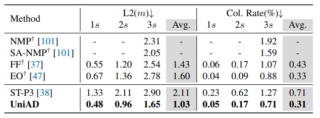
Fig 23. Planning results. [6]
References
[1] Zhang, Qihang, et al. “Learning to Drive by Watching YouTube Videos: Action-Conditioned Contrastive Policy Pretraining.” European Conference on Computer Vision. 2022.
[2] He, Kaiming, et al. “Momentum Contrast for Unsupervised Visual Representation Learning.” Proceedings of the IEEE/CVF Conference on Computer Vision and Pattern Recognition (CVPR). 2020.
[3] Sima, Chonghao, et al. “DriveLM: Driving with Graph Visual Question Answering.” arXiv. 2023.
[4] Brohan, Anthony, et al. “RT-2: Vision-Language-Action Models Transfer Web Knowledge to Robotic Control.” arXiv. 2023.
[5] Levine, Sergey, et al. “End-to-End Training of Deep Visuomotor Policies.” Journal of Machine Learning Research. 2016.
[6] Hu, Yihan, et al. “Planning-oriented Autonomous Driving.” Proceedings of the IEEE/CVF Conference on Computer Vision and Pattern Recognition (CVPR). 2023.
[7] Li, Zhiqi, et al. “Panoptic SegFormer: Delving Deeper into Panoptic Segmentation with Transformers.” Proceedings of the IEEE/CVF Conference on Computer Vision and Pattern Recognition (CVPR). 2022.
[8] Zhu, Xizhou, et al. “Deformable DETR: Deformable Transformers for End-to-End Object Detection.” arXiv. 2020.
[9] Li, Junnan et al. “BLIP-2: Bootstrapping Language-Image Pre-training with Frozen Image Encoders and Large Language Models.” Proceedings of the 40th International Conference on Machine Learning. 2023.
[10] Li, Zhiqi et al. “BEVFormer: Learning Bird’s-Eye-View Representation from Multi-Camera Images via Spatiotemporal Transformers.” European Conference on Computer Vision. 2022.
[11] Zeng, Fangao et al. “MOTR: End-to-End Multiple-Object Tracking with Transformer.” European Conference on Computer Vision. 2022.
[12] Carion, Nicolas et al. “End-to-End Object Detection with Transformers.” European Conference on Computer Vision. 2020.