Depth Estimation

Depth estimation is defined as the computer vision task of calculating the distance from a camera to objects in a scene. It has become more and more important, with a wide variety of applications in many fields, including autonomous vehicles, medicine, and human-computer interaction. Recent deep learning methods have enhanced the accuracy, robustness, and efficiency of depth estimation methods in both images and videos. We discuss two different deep learning approaches to depth estimation, including an Unsupervised CNN, and Depth Anything. We compare and contrast these approaches, and expand on the existing code by combining it with other effective architectures to further enhance the depth estimation capabilities.

• Introduction
• Unsupervised CNN for Single View Depth Estimation
  • Implementation:
  • Results and Discussion
• Depth Anything: Unleashing the Power of Large-Scale Unlabeled Data
  • Motivation
  • Approach
  • Architecture
  • Datasets and Training Pipeline
  • Results
• Comparison
• Code
  • Demo
• Conclusion
• References

Introduction

Depth estimation has become more and more popular, as it has a variety of applications in many distinct fields. It is fundamental to understanding the 3D structure of any space, which is useful for object manipulation, navigation, and planning. Depth estimation can help improve the decision making process of both humans and robots, as knowing the spatial relationship between objects within an environment allows for more informed decisions. Depth estimation also provides analytical capabilities. It allows for the extraction of meaningful data from visual information, which can be used to analyze patterns, detect anomalies, and predict trends in countless domains, enhancing the ability to derive actionable insights from visual inputs.

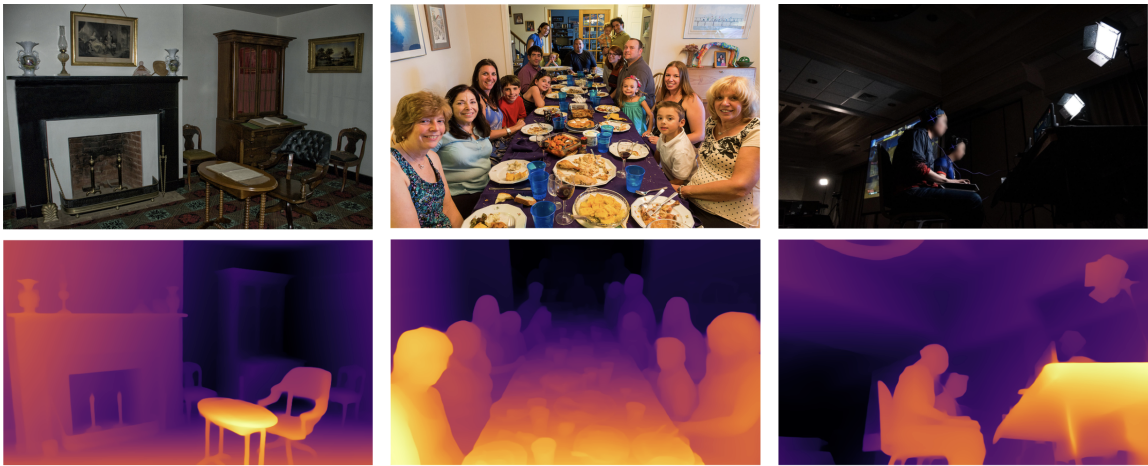
Figure 1: Example of Depth Estimation [1]

This is an example of depth estimation from an image input. As we can see in the center image, the people closer to the sensor or camera are more brightly highlighted, while the people in the background have less emphasis on them. Depth estimation isn’t only limited to certain objects, as it estimates the depth of the walls, floor, and everything else in the image. There are two main types of depth estimation: Monocular, where only a single input view is taken in, and stereo, where a pair of images is inputted, and using differences between the two images, a depth estimation is outputted. Both are widely used, and each have their own advantages. Monocular images are much easier to obtain, not requiring a paired camera setup. However, there are techniques that we can only do a stereo pair that could more accurately estimate depth.

Depth estimation has applications in robotics, augmented reality, and human-computer interaction, among countless other fields. With the advent of self-driving cars, depth estimation is incredibly important to allow these autonomous vehicles to detect nearby cars or pedestrians, and adjust accordingly. Additionally, augmented reality uses depth estimation to correctly place objects in an unfamiliar 3D space. For example, IKEA has a demo where customers can visualize IKEA products in their own home through AR, before purchasing them. The furniture is projected into a 3D space through depth estimation. Finally, depth estimation can help us gain a better understanding of human-computer interaction, specifically human gestures and movements. It also has applications in portrait mode pictures, object trajectory estimation, and so much more. We will explore two approaches towards depth estimation, the first being a Convolutional Neural Network for Single View Depth Estimation.

Unsupervised CNN for Single View Depth Estimation

CNNs have been a staple in the deep learning community for years, and have been used for a variety of tasks, including image classification, object detection, and now depth estimation. The premise behind this paper was the weakness of requiring massive amounts of labeled data to train deep CNNs. In Unsupervised CNN for Single View Depth Estimation, the primary solution to the lack of training data for monocular depth estimation is to train a CNN-based encoder on unlabeled stereoscopic image pairs. This encoder is optimized by minimizing the error between the left image and a reconstruction of that image via inverse warping of the right image and the predicted depth map. It performs similarly to many supervised learning methods, but requires no manual annotations or labeled data.

Implementation:

In order to train the network, a pair of images with a known camera displacement between them, such as a stereo pair, is fed in. These images don’t require any labels, and thus are significantly easier to obtain compared to depthmaps. A CNN learns the conversion from image to depth map. It is trained using the photometric loss between the source image (one of the two input images), and the inverse warped target image, the other image in the input pair. This loss is differentiable, allowing the model to perform backpropagation. This process is similar to the autoencoders discussed in class, with one key difference. Their model encodes the source image into a depth map, but instead of learning a decoder, uses a standard geometric operation of inverse warping to reconstruct the input image. This allows the decoder training process to be skipped, while still accurately estimating the depth of input images.

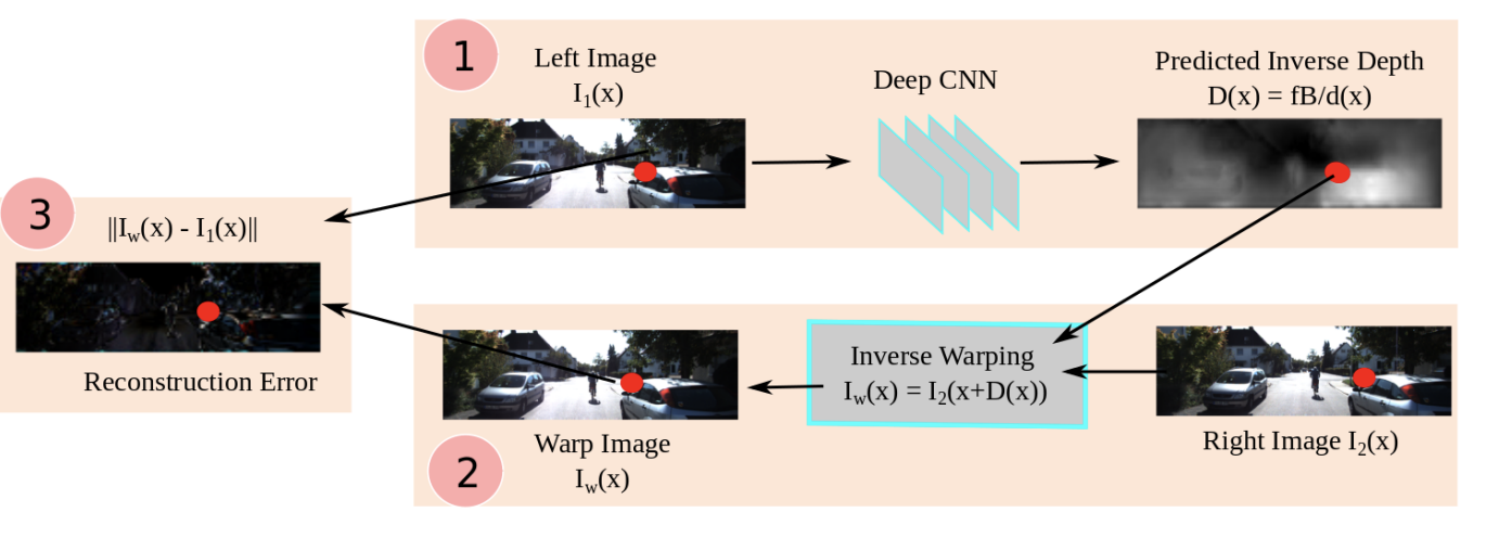
Figure 2: Unsupervised CNN structure [2]

We can see a general setup of the implementation in Figure 2. In part 1, the encoder CNN maps the left image of the input pair to a predicted depth map. In part 2, the decoder creates a warped image by using an inverse warping from the right image of the input pair and the depth map, along with the known displacement between the two input images. The reconstructed output and the original input are then used to calculate the loss and train the network. At test time, we solely use the encoder, and predict the depthmap for a single-view image.

Autoencoder Loss:

The input images are captured by a pair of cameras. Let \(f\) be the focal length of the camera, and \(B^2\) is the horizontal distance between the two cameras. Additionally, let the predicted depth of pixel \(x\) in the left input image be \(d^i(x)\). The motion of a pixel along a line from the left image to the right image is then \(fB/di(x)\). Applying this to all pixels in the left image, we can get a warping \(I^i_w\) from the left image to a reconstruction through the right image \(I^i_2\) and depth map: \(I^i_w = I^i_2(x + fB/di(x))\). Using this warping, we compare it to the original image to get our reconstruction loss, as shown in equation 1.

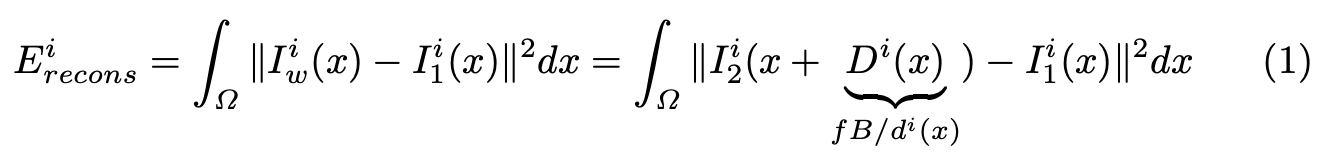
Equation 1: Autoencoder loss [2]

The paper also added an additional regularization term, in order to deal with something known as the aperture problem: the reconstruction loss is inaccurate when there are very similar regions in the same scene. This value, shown in Equation 2, is combined with the reconstruction loss to generate the full autoencoder loss, in Equation 3. The smoothness prior strength hyperparameter was set to 0.01.

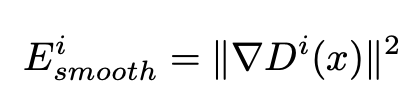
Equation 2: Regularization term [2]

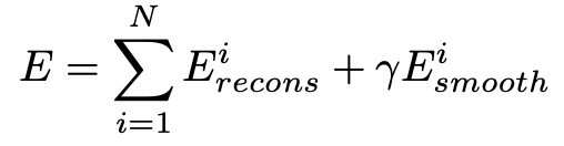
Equation 3: Total Loss [2]

Coarse to Fine Training

Using a Taylor expansion to linearize the loss function as shown in equation four allows the loss to be backpropagated. This Taylor equation is shown in Equation 4.

Equation 4: Taylor Expansion of Loss [2]

In this case, \(I_{2h}\) represents the horizontal gradient of the warped image, computed at disparity \(D^{n-1}\). This only works when the difference in disparities \((D^n(x) - D^{n-1}(x))\) is small. To estimate larger disparities, the paper implements a coarse-to-fine architecture, along with iterative warping of the input image. To do this, a robust disparity initialization at the finer resolutions to linearize warps is needed, along with the corresponding CNN layer which predict the initial disparities. The paper uses a fully convolutional network, or FCN, to do this upsampling.

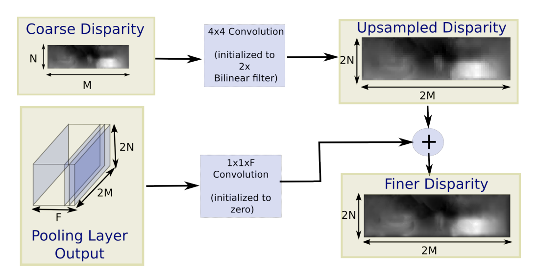
Figure 3: CNN Upsampling [2]

As shown in Figure 3, given an input of Coarse Disparity, a bilinear upsampling filter is used to initialize upscaled disparities, which is double the size of the input. Finer details of the images are captured in the previous layers of CNN from the downsampling part, and combining the upscaled and finer disparities are helpful for refining the prediction. To do this, a 1 × 1 convolution initialized to zero is used, and then the convolved output is combined with the bilinear upscaled depths through an element-wise sum, in order to get our final refined disparity map.

Architecture and Code Implementation

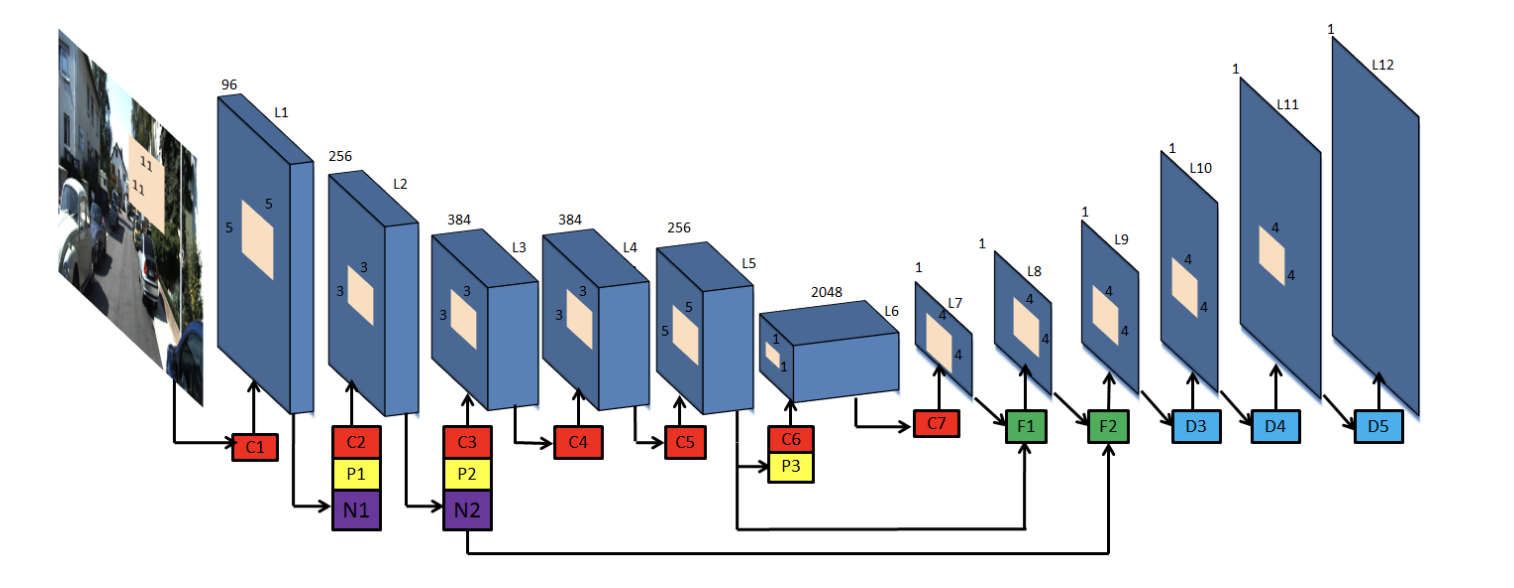
Figure 4: CNN Architecture [2]

The architecture of the encoder CNN is shown in Figure 4. It is similar to the first five layers of AlexNet [4] , up to the C5 layer. These compose of convolutional and pooling layers, along with a ReLU activation function. The initial input is a 227x227x3 RGB image. Each convolutional layer takes in the image, and transforms it based on the number of channels. For the first two layers, there is also a LocalResponseNorm layer, which normalizes the pixel values within a small neighborhood of pixels, in this case the neighborhood is defined to be across the channels. The first five layers compose of five convolutional layers, 2 max pooling layers, and 2 normalization layers in total.

self.net = nn.Sequential(
    nn.Conv2d(in_channels=3, out_channels=96, kernel_size=11, stride=4),  # (b x 96 x 55 x 55)
    nn.ReLU(),
    nn.LocalResponseNorm(size=5, alpha=0.0001, beta=0.75, k=2),  # section 3.3
    nn.MaxPool2d(kernel_size=3, stride=2),  # (b x 96 x 27 x 27)
    nn.Conv2d(96, 256, 5, padding=2),  # (b x 256 x 27 x 27)
    nn.ReLU(),
    nn.LocalResponseNorm(size=5, alpha=0.0001, beta=0.75, k=2),
    nn.MaxPool2d(kernel_size=3, stride=2),  # (b x 256 x 13 x 13)
    nn.Conv2d(256, 384, 3, padding=1),  # (b x 384 x 13 x 13)
    nn.ReLU(),
    nn.Conv2d(384, 384, 3, padding=1),  # (b x 384 x 13 x 13)
    nn.ReLU(),
    nn.Conv2d(384, 256, 3, padding=1),  # (b x 256 x 13 x 13)
    nn.ReLU(),
        )

Instead of the last maxpooling layer after C5, and then a sequence of fully connected layers, the encoder CNN uses 2048 convolutional filters, each of size 5x5 [3]. This reduces the number of parameters in the network, as convolutional layers are much cheaper than fully connected ones. It also enables the network to accept input images of varying sizes. Finally, we pass it through one more 1x1 convolutional layer, that allows us to get one channel for the predicted depth map. Then, the model starts sequentially upsampling the predicted depth map, at first using bilinear interpolation, to allow the final prediction to be detailed and match the original input size. The model preserves spatial information within the image. Note that we also combine the output of layers L3 and L5 with the upsampling from F1 and F2, in order to combine the coarser depth prediction with the local image information.

self.fcn = nn.Sequential(
    nn.Conv2d(in_channels=256, out_channels=2048, kernel_size=5),  # C6
    nn.ReLU(),
    nn.MaxPool2d(kernel_size=3, stride=2),  
    nn.Conv2d(in_channels=2048, out_channels=1, kernel_size=1),  # C7
    nn.ReLU(),
    nn.Upsample(scale_factor = 2, mode=’bilinear’),  # F1
    nn.ReLU(),
    nn.Upsample(scale_factor = 2, mode=’bilinear’),  # F2
    nn.ReLU(),
)

We then use transposed convolution in order to upsample the output to the original dimensions of the input, so that we can compare them and accurately calculate the reconstruction loss. The transposed convolution uses 4x4 kernels, as well as a stride of 2, and a padding of 1. The image dimensions end up in 176 x 608, which is the same as the input image dimensions.

self.upsample = nn.Sequential(
    nn.ConvTranspose2D(1, 1, kernel_size=4, stride=2, padding=1),  # D3, 44 x 152
    nn.ReLU(),
    nn.ConvTranspose2D(1, 1, kernel_size=4, stride=2, padding=1),  # D4, 88 x 304
    nn.ReLU(),
    nn.ConvTranspose2D(1, 1, kernel_size=4, stride=2, padding=1),  # D5, 176 x 608
    nn.ReLU(),
)

The model was trained on the KITTI dataset, a well known dataset for depth estimation on outdoor scenes of stereo image pairs. From the 56 scenes within the city, residential, and road categories, they split it in half for training and testing. They downsample the left input image to 188 x 620, and input them into the network. The right images are downsampled and used to generate warps at each of the predicted depthmap stages(L8-L12). Around 22,000 total images were used for training, and 1,500 images for validation. Instead of using ground truth labels, the paper upscales the low resolution disparity predictions to the resolution at which the stereo images were captured to evaluate the model. Notably, this doesn’t require any manual annotations or labeled data, allowing for a much quicker and easier training process. Using the stereo baseline of 0.54 meters for D, ground truth depthmaps at resolution can be generated using d = fB/D, through the upsampled disparities. The evaluation metrics on the model are shown in equation 5.

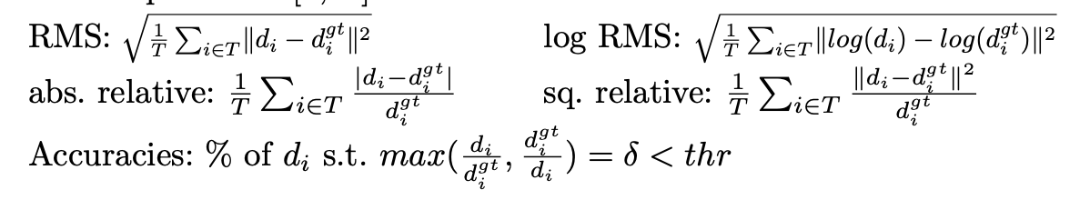
Equation 5: Evaluation Metrics [2]

RMS is the difference in depth between the depth prediction and ground truth squared and then averaged and square rooted. Log RMS is similar, but takes the log of the prediction and ground truth first. Relative errors divide by the ground truth label. Finally, they evaluate the number of depth predictions such that the difference in prediction is under some threshold, meaning that it is relatively similar to the ground truth.

SGD with momentum of 0.9 and weight decay of 0.0005 was used for the optimizer. Network weights were initialized randomly for layers C1 to C5, and for the 5x5 convolution, weights were set to 0 in order to get 0 disparity estimates. The pixel values are normalized such that all values are between -0.5 and 0.5. The learning rate for starts at 0.01 for the coarsest resolution predictions, and gradually decreases based on the equation \(lr_{t-1} = lr_t * 1/(1 + αn) (n−1)\), where n is the index of current epoch and α = 0.0005. The model is trained for 100 epochs.

Further augmentation was done while fine tuning the model: Color channels were multiplied by a random value between 0.9 and 1.1, the input image was upscaled by a random factor between 1 and 1.6, and the left and right input images were swapped, in order to enable the model to learn new training pairs with positive disparity. This lead to noticeable improvements, as shown below.

Results and Discussion

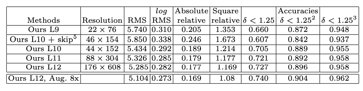
Table 1: Performance With Upsampling [2]

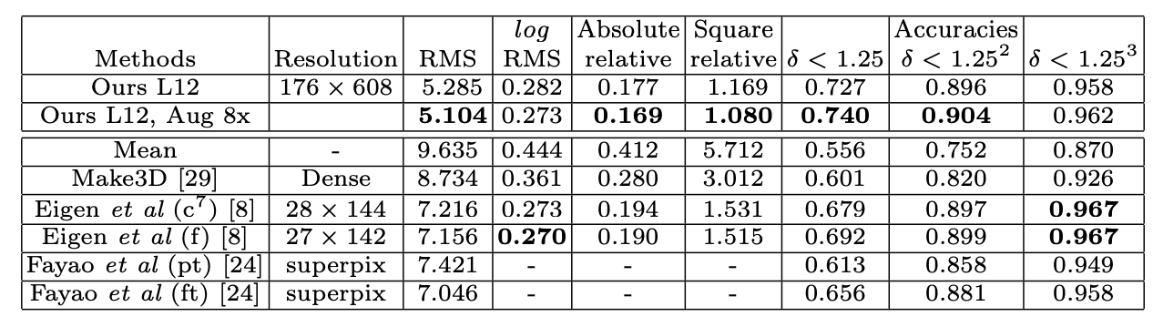
Table 2: Performance Compared with Supervised Learning Methods [2]

In Table 1, we see the performance of their model at different resolutions. In each subsequent layer, the output depth map is upsampled by a factor of 2, and there is clearly a correlation between resolution and performance, as all error and accuracy metrics improve as resolution increases. It is interesting to consider how further upsampling may have affected the performance. In Table 2, the performance of their model compared to state of the art supervised learning methods is shown. It is clear that this unsupervised learning method is on par with, or even outperforms other supervised learning methods in a variety of metrics. Even with random initialization of weights and no ground truth labels, the model is still able to perform well.

Figure 5: Output with and without Augmentation [2]

Figure 5 shows an actual example of the outputted depth map. Note that the colors are brighter when the object is closer to the camera, and the depth map is able to capture much more detail. Even though this output now looks pretty low quality, at the time for an unsupervised method, it was considered quite effective. The results with the augmentations described above were able to localize object edges better, an important feature of depth estimation. Fine tuning significantly improved the results at a cheap training cost, and could be expanded to new outdoor datasets or perhaps other scenes as well.

One main downside of this approach is that it still needs focal length and paired input images in order to estimate depth effectively. Additionally, while this model was impressive for its time in 2017, architectures have only gotten deeper and more powerful, and what was considered a good depth estimation before is now significantly lower quality when compared to current state of the art methods. In the next section, we discuss a much more modern and powerful approach to monocular depth estimation.

Depth Anything: Unleashing the Power of Large-Scale Unlabeled Data

Motivation

The motivation behind Depth Anything is similar to above where it is difficult to obtain a large depth-labeled dataset. This is addressed by scaling up and annotating a wide variety of unlabeled data images and augments with a smaller set of labeled data images to provide a robust annotation tool.

Approach

The general approach of Depth Anything (as shown below) is to first train a MiDaS-based monocular depth estimator on images labeled with their corresponding depth maps. Once this model is trained, it then serves as a teacher model which is used to predict the depth maps of unlabeled images. These predicted depth maps can then be used as the labels of the corresponding images, essentially yielding a new set of pseudo-labeled images. Next, a student model, which consists of a pre-trained DINOv2 encoder and a DPT decoder, is trained both on the available labeled data as well as the pseudo-labeled pictures. To create a more robust training set, additional data augmentations are also introduced to the pseudolabeled images such as color jittering, gaussian blur, and cutmix spatial distortion. Finally, the Depth Anything model is trained to learn/encode semantic segmentation information about the unlabeled/pseudolabeled image set. This serves to provide additional context that could help the model differentiate between objects when predicting a depth map for the image.

Architecture

Diving into the architecture, the DINOv2 encoder has been trained previously to capture features that are semantically meaningful in the images and will be fine-tuned further. The decoder consists of projection layers, resizing layers, feature fusion blocks, upsampling and refinements blocks, and output convoluational layers.

The projection layers modify the channel dimension of each feature map to a consistent size suitable for fusion and by creating a series of 1x1 convolutional layers, each with a different number of output channels as specified in the out_channels list.

        self.projects = nn.ModuleList([
            nn.Conv2d(
                in_channels=in_channels,
                out_channels=out_channel,
                kernel_size=1,
                stride=1,
                padding=0,
            ) for out_channel in out_channels
        ])

The resizing layers consist of a combination of transposed convoluations, identity mappings, and regular convulations to resize the feature maps to higher resolutions at different stages within the network.

self.resize_layers = nn.ModuleList([
            nn.ConvTranspose2d(
                in_channels=out_channels[0],
                out_channels=out_channels[0],
                kernel_size=4,
                stride=4,
                padding=0),
            nn.ConvTranspose2d(
                in_channels=out_channels[1],
                out_channels=out_channels[1],
                kernel_size=2,
                stride=2,
                padding=0),
            nn.Identity(),
            nn.Conv2d(
                in_channels=out_channels[3],
                out_channels=out_channels[3],
                kernel_size=3,
                stride=2,
                padding=1)
        ])

The feature fusion blocks merge features from different layers to maintain fine-grained information at various scales, potentially enhancing its ability to capture and represent complex patterns in the data. Residual units are also used here when applying a series of convolutions to maintain robustness and stability in training. In summary, this code sets up a series of feature fusion blocks within a neural network architecture.

class FeatureFusionBlock(nn.Module):

…

        self.out_conv = nn.Conv2d(features, out_features, kernel_size=1, stride=1, padding=0, bias=True, groups=1)

        self.resConfUnit1 = ResidualConvUnit(features, activation, bn)
        self.resConfUnit2 = ResidualConvUnit(features, activation, bn)
        
        self.skip_add = nn.quantized.FloatFunctional()

…

Finally, the output convolutional layers are applied to reach a final output to produce either a multiclass segmentation map or a single-channel depth map, depending on the task at hand. The use of different layers and configurations allows the network to be flexible and applicable to different types of tasks, such as semantic segmentation or depth estimation.

        if nclass > 1:
            self.scratch.output_conv = nn.Sequential(
                nn.Conv2d(head_features_1, head_features_1, kernel_size=3, stride=1, padding=1),
                nn.ReLU(True),
                nn.Conv2d(head_features_1, nclass, kernel_size=1, stride=1, padding=0),
            )
        else:
            self.scratch.output_conv1 = nn.Conv2d(head_features_1, head_features_1 // 2, kernel_size=3, stride=1, padding=1)
            
            self.scratch.output_conv2 = nn.Sequential(
                nn.Conv2d(head_features_1 // 2, head_features_2, kernel_size=3, stride=1, padding=1),
                nn.ReLU(True),
                nn.Conv2d(head_features_2, 1, kernel_size=1, stride=1, padding=0),
                nn.ReLU(True),
                nn.Identity(),
            )

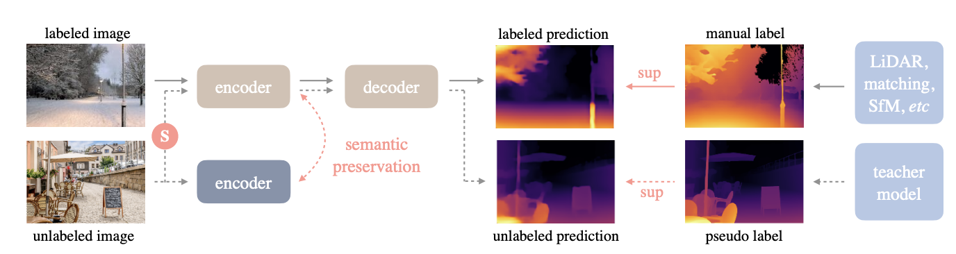
Figure 6: Depth Anything Model Structure [1]

Student Model Cost Functions

During training of the student model, Depth Anything minimizes on the average of three loss functions, each evaluating the accuracy of one aspect of the model.

1. Labeled Data

The first loss function helps optimize the performance of the model when inferring on labeled data.

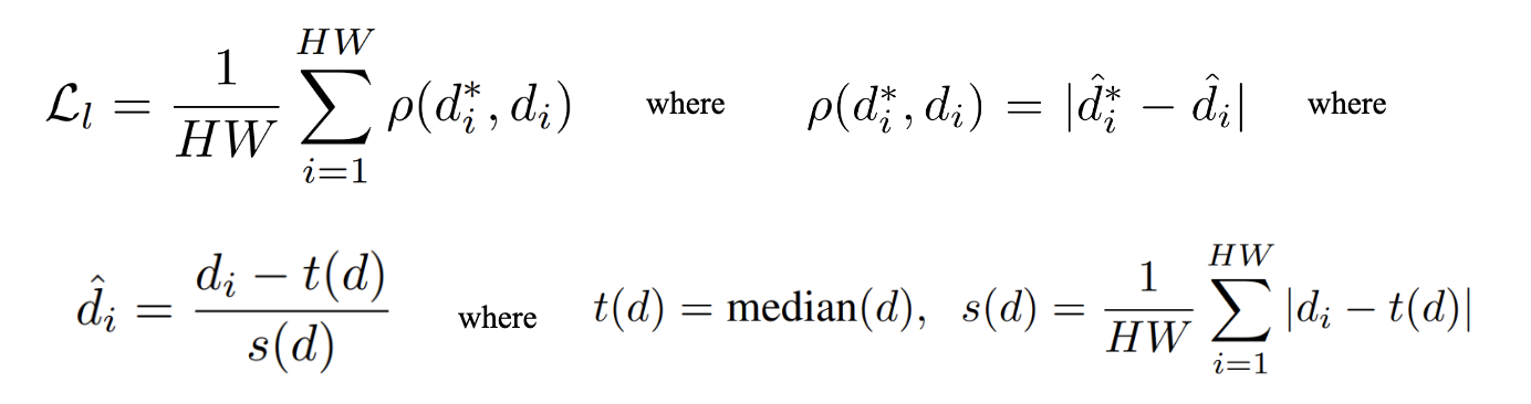
Equations 6-9: Affine-Invariant Mean Absolute Error [1]

As shown in the equations above, the first loss function measures the affine-invariant mean absolute error between the predicted deaths and the ground truth depth. First, as seen in Equation 8 and 9, the predicted depth values are shifted by the median and scaled by the mean absolute deviation of disparities over all pixels in the predicted depth map of a particular labeled example. The ground truth depth values also undergo the same transformations, except they are shifted and scaled by the statistics of the ground truth depth map. This makes both the predicted and actual depth maps affine-invariant, since all depth values now have a distribution of median 0 and absolute deviation 1 (regardless of how depths may have been scaled or shifted from example to example). Finally, as seen in equation 6 and 7, the absolute error between the normalized depth values of each corresponding pixel predicted and ground truth depth map is then calculated, before being averaged over all pixels in the image.

This first loss function is minimized to improve the pixel-by-pixel accuracy of the model’s predicted depth values compared to the actual depth values. By making it affine-invariant, the loss is not biased towards examples that may have depth values that are larger in scale.

2. Unlabeled Data

The second loss function helps optimize the performance of the model when inferring on augmented pseudolabeled data. Before discussing the loss function itself, let’s explore the data augmentation techniques explored in Depth Anything.

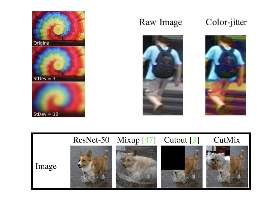
Figure 7: Gaussian Blurring (top left), Color Jittering (top right), CutMix Data Augmentation (bottom) [1]

As seen in figure 7, two types of color distortion are added to the unlabeled images. The first is Gaussian blur, in which a Gaussian distribution is convolved over an image to blur the edges and feature of the image. The second is color jitter, in which an image’s brightness, contrast, saturation, and hue are randomly changed. These two types of image augmentation do not actually affect the positions or values of the ground truth depths of the image (at any given pixel in the image, the actual depth is still the same even after the augmentation). Thus, they can be evaluated on the same loss function as for labeled data.

The third type of image augmentation used was CutMix, which is a type of spatial distortion. A rectangular section is taken out of one training image, and then replaced with the corresponding section of a different image. Since the corresponding ground truth depth map is different after CutMix (taking into account the depth maps of both images used), the cost function must be modified, as discussed in the next section.

Image augmentation helps the student model be more robust to unseen images. It adds perturbations that make the depth map prediction task more difficult given the more surface-level features of the image. Instead, the model is forced to “actively seek extra visual knowledge and acquire invariant representations from these unlabeled images.” This extra information is more generalizable across different types of images, thus improving the performance of the model on images in new domains that it may not have been trained on.

Taking a look at the loss function used for training on unlabeled/pseudolabeled data:

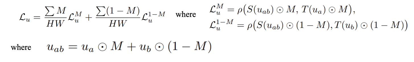
Equations 10-13: Affine-Invariant Mean Absolute Error, Accounting for Cutmix Augmentations [1]

In equation 11, \(ρ\) describes the same affine-invariant absolute error function as the one introduced in equation 7. The difference is what is passed in as the arguments to ρ. Since images that have undergone CutMix will have pixels associated with different images/depth maps at different pixels, we must first determine which ground truth depth map to evaluate at each pixel of the image, before passing the predicted depth along with the ground truth depth value at that pixel into \(ρ\). In all three of the above equations, \(M\) is a binary mask over the entire image with 0 corresponding to original image and 1 corresponding to the “cut-in” image, thus masking out the original image. It follows that \(1- M\) masks out the “cut-in” image. \(u_{ab}\) is the RGB values of the pixels of the image after CutMix is applied with image a being cut into image b. For the pixels in the cut-in region, \(L^M_u\) is the affine-invariant mean absolute error between the student model depth prediction and the teacher model depth prediction (pseudo-label) for image \(a\), For the pixels in the other part of the image, \(L^{1-M}_u\) is the affine-invariant mean absolute error between the student model and teacher model depth prediction for image \(b\). We then take the weighted average of both losses to calculate the final loss.

3. Semantic Segmentation Feature Alignment Loss

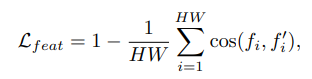
Equation 14: Feature Alignment Loss [1]

Finally, the paper proposed adding semantic segmentation data as an input to the student model to help improve performance, since it would help add additional context for depth estimation and also reduce pseudo label noise. The paper found that simply adding this data doesn’t improve the model by much, so instead they optimized the student model on feature alignment loss between the output of the Depth Anything encoder and a frozen DINOv2 encoder on a pixel of a training image. The base DINOv2 encoder, as mentioned previously, captures semantically significant visual features in the image. Thus, by ensuring the DepthAnything a feature vector similar to DINOv2’s, this ensures DepthAnything is learning semantic information about the image as well that could be used to differentiate between objects in the scene of the image.

Looking at the actual loss function, the feature alignment loss is essentially one minus the cosine similarity between a DepthAnything encoder feature vector and the DINOv2 encoder feature vector. Again, by minimizing the feature alignment loss, we are ensuring that our Depth Anything model learns some semantic segmentation information about the image. However, to prevent overfitting on the semantic segmentation task, if the similarity between two feature vectors for a certain pixel is too high, DepthAnything will not consider it in the feature alignment loss.

As mentioned at the beginning, the student model is trained by optimizing an average of all three losses.

Datasets and Training Pipeline

Depth Anything leverages both labeled and unlabeled data to train its teacher model. The labeled images come from the following datasets:

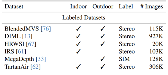
Table 3: Labeled Datasets Used by DepthAnything [1]

As can be seen in table 3, most of the labeled data comes from stereo datasets containing pairs of images labeled with their ground truth depth maps. Since the teacher MiDaS model and student Depth Anything model are both monocular depth estimators, these labeled datasets are repurposed as monocular datasets by only considering one image/depth map per example. Larger, more common datasets like KITTI and NYUv2 are used to evaluate zero-shot learning, so DepthAnything employs less common datasets for training such as BlendedMVS, which contains images and depth maps of indoor and outdoor scenes, and DIML, which contains Kinect-captured indoor and outdoor images. The total number of images in this collection is around 1.5 million.

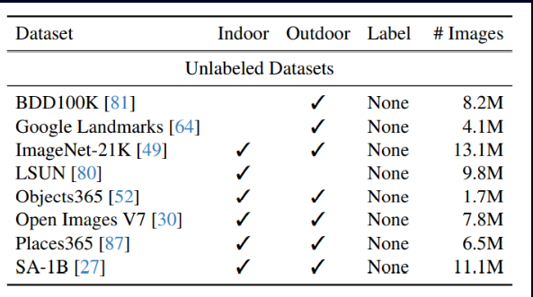
Table 4: Unlabeled Datasets Used by DepthAnything [1]

As can be seen in table 4, the unlabeled data comes from large datasets of images, most of which are labeled for tasks other than depth estimation. For example, Google Landmarks is a set of images of landmarks labeled with the actual names of the landmarks. ImageNet contains images of everyday objects and is labeled with the identity of those objects. Because these datasets are intended as unlabeled data, the labels can simply be ignored. By removing the need to have images labeled specifically with depth maps, there is a larger abundance of image datasets to sample from, allowing Depth Anything to take advantage of 65 million unlabeled images.

Training the teacher model:

The teacher model is run through 20 epochs of training with layer-specific learning rates. The encoder utilizes a learning rate of \(5 * 10^{-6}\), while the decoder is trained with a learning rate of \(5 * 10^{-5}\). Finally, the optimizer used for training is AdamW with linear learning rate decay. AdamW is an evolution of Adam that optimizes weight decay separately from learning rate decay.

Training the student model:

To train the student model, pseudo-labels are first assigned to each unlabeled image by running the image through the teacher model to generate a predicted depth map. Next, labeled and pseudo-labeled data is split into batches with a 1:2 ratio between the number of labeled and the number of unlabeled images. Until all pseudo-labeled images are exhausted, the student model is then trained on the batches with the same layer-specific learning rates, optimizer, and learning rate decay as the teacher model. Finally, labeled images have horizontal flipping applied during training, and for feature alignment loss, pixels with a loss (1 - cosine similarity) of less than 0.15 are omitted from the cumulative loss.

Results

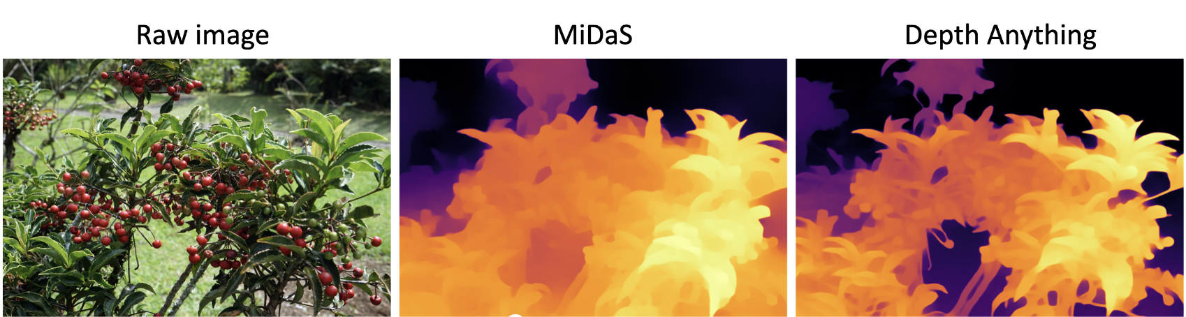
Figure 8: Example of Depth Anything Output [1]

Above is an example picture of the depth estimation produced by Depth Anything vs. the previous most known model for molecular depth estimation. It is quite evident that the Depth Anything image was able to abstract and define clearly between the various objects of different depths, meanwhile the other models blurs the areas where there tend to be changes in depths. Overall Depth Anything image looks much sharper and extracts the most depth information from the raw image.

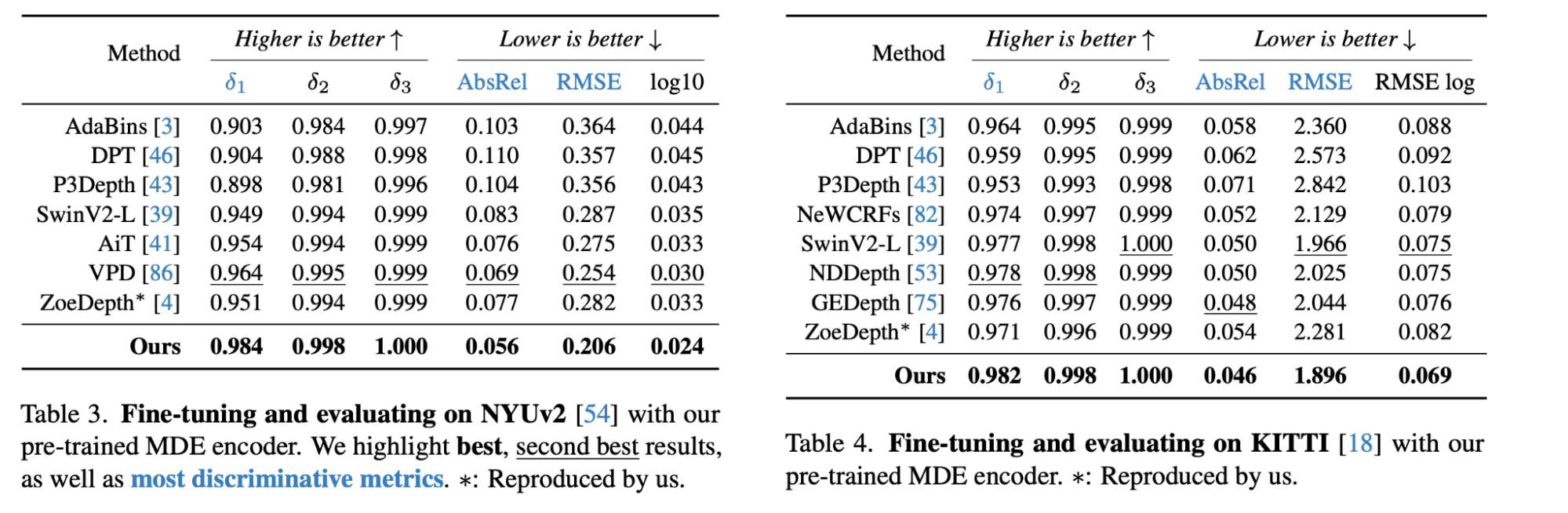
Tables 5 and 6: Comparison between Depth Anything and other Methods on in-domain Datasets [1]

In the figure above, it shows how Depth Anything produces better results in-domain estimation compared to other novel depth estimations models with better scores in δ and absolute relative error as well as root mean squared error.

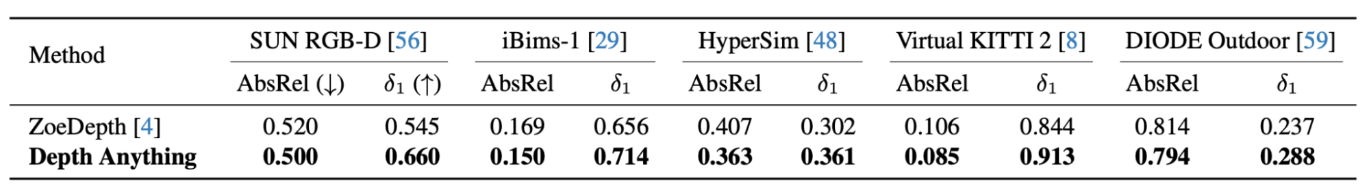
Table 7: Comparison between Depth Anything and ZoeDepth on zero-shot Learning [1]

In the figure above, it shows how Depth Anything produces better results for zero-shot metric depth estimation on various datasets as well than the previously metric molecular depth estimation model ZoeDepth.

Comparison

In Unsupervised CNN for Single View Depth Estimation, the primary solution to the lack of training data for monocular depth estimation is to train a CNN-based encoder on unlabeled stereoscopic image pairs. This encoder is optimized by minimizing the error between the left image and a reconstruction of that image via inverse warping of the right image and the predicted depth map. This means that there is no need for labeled data as the model exploits geometric consistency between the left and right images, which is a natural cue in depth perception. However, this system is still dependent on the availability of stereo pairs, which are far less common than single-view photos. Furthermore, a reconstructed image may not perfectly match the original left image, especially in regions with occlusions and complex textures, which can easily affect the depth estimation. The smoothness assumption prior on disparities may not always hold true either in real-world scenes that contain sharp depth discontinuities and would lead to oversmoothed depth maps. Depth Anything proposes a system in which an MDE can be trained on a combination of labeled and unlabeled monocular images. This enables the depth estimator to be trained on datasets of images that can be easily obtained and expanded upon. Both are unsupervised and endeavors to resolve the significant issue of a lack of training data.

After observing both the the result tables for both models when trained on the KITTI dataset, it seems that the δ accuracies Depth Anything (0.982, 0.998, 1.00) performs better than the Unsupervised CNN for Single View Depth Estimation (0.740, 0.904, 0.962). The absolute relative error and root mean squared error of Depth Anything (0.46, 1.896) is better than Unsupervised CNN for Single View Depth Estimation (0.169, 5.104). Overall Depth Anything still outperforms Unsupervised CNN for Single View Depth Estimation most likely evident to the fact that Depth Anything used more modern ideas as the paper was just published this year as opposed to Unsupervised CNN for Single View Depth Estimation published back in 2017. Depth Anything was trained on a combination of labeled and unlabeled monocular images as well as utilized more complex data augmentation algorithms such as CutMix, allowing for a more diverse, robust, and extensive training dataset. This likely helped the model to learn more generalizable features for depth estimation, compared to relying solely on unsupervised learning and stereoscopic pairs. Unsupervised CNN for Single View Depth Estimation utilizes some level of feature combination in combining of different convolution and upsampling layers to integrate coarser depth predictions with local image information. On the other hand, Depth Anything employs more advanced model architecture such as Feature fusion blocks with residual connections to fuse features from different layers of network to provide a richer representation of the scene. This allows the model to better distinguish between continuous surfaces and discontinuities allowing for sharper output images.

Code

We finetuned the Depth Anything model for a downstream task in order to do image classification. We explored fine tuning the model on the Miniplaes dataset we used in Assignment 2. We also explore running the Depth Anything model on our own images, and evaluating the generated depthmap. Unfortunately, due to the Depth Anything authors not providing their source model, we were unable to make modifications and train it from scratch. None of the teacher model code is included in the Github. It only contains the pretrained model, which we then used to finetune for an image classification model.

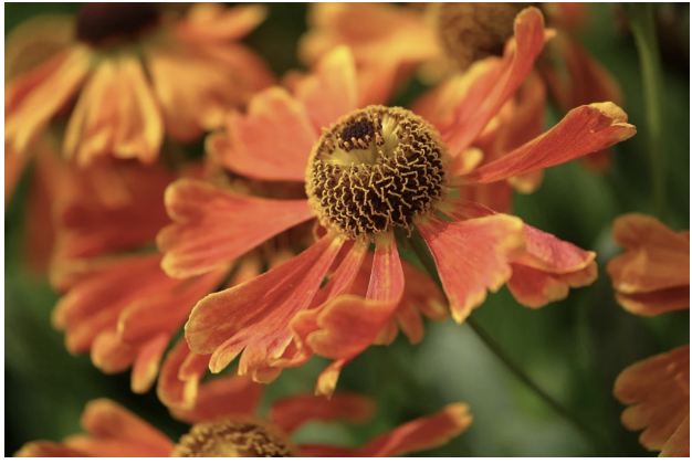
Figure 9: Sample Image

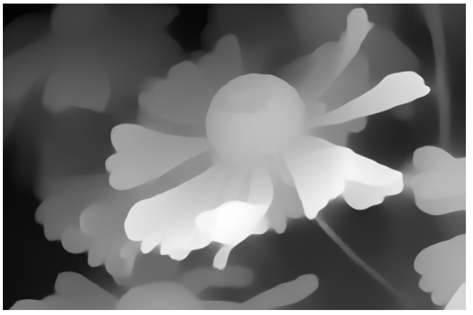
Figure 10: Sample Depthmap

We can see an example of a Depth Anything depthmap in figure 10, from the original image in figure 9. As we can see, the closer the object is to the camera, the more bright it is. Note how Depth Anything can also capture the flowers in the background as well in detail.

Demo

First, in order to finetune the model, we clone the repository from github.

!git clone https://github.com/LiheYoung/Depth-Anything.git
%cd Depth-Anything

Import the required libraries, such as torch, numpy, and more.

import cv2
import numpy as np
import torch
import torch.nn.functional as F
import torchvision.models as models
from torch import nn

Then, download a dataset of your choice. In our demonstration, we use the miniplaces dataset.

# Downloading this file takes about a few seconds.
# Download the tar.gz file from google drive using its file ID.
!pip3 install --upgrade gdown --quiet
# unfortunately, only the following command seems to be constantly working...
!wget https://web.cs.ucla.edu/~smo3/data.tar.gz

Follow the same steps as the assignment, or follow the instructions for your own dataset. After the dataset is downloaded into colab, we can set up the model.

from depth_anything.dpt import DepthAnything




class DepthAnythingFinetuned(nn.Module):


   def __init__(self, include_residual=True):
       super().__init__()


       encoder = 'vits' # can also be 'vitb' or 'vitl'


       # config = {"encoder":'vitl', "features":256, "out_channels":[256, 512, 1024, 1024], "use_bn":False, "use_clstoken":False, "localhub":False}


       input_channels = 4 if include_residual else 1
       self.depth_anything = DepthAnything.from_pretrained('LiheYoung/depth_anything_{:}14'.format(encoder), local_files_only=False)
       self.cnn = FastConv(input_channels=input_channels,
                conv_hidden_channels=64,
                conv_out_channels=128,
                input_size=(140, 140),
                dropout_rate1=0.25,
                dropout_rate2=0.5,
                fc_out_channels=128,
                kernel_size=3,
                stride=2,
                padding=1,
                num_classes=len(miniplaces_train.label_dict))
       self.include_residual = include_residual
       # self.depth_anything_conv = nn.Sequential(self.depth_anything, self.cnn)


   def forward(self, x):
       if self.include_residual:
         res = x
         x = self.depth_anything(x)
         x = torch.reshape(x, (x.shape[0], 1, x.shape[1], x.shape[2]))
         x = torch.concat((res, x), 1)
       else:
         x = self.depth_anything(x)
         x = torch.reshape(x, (x.shape[0], 1, x.shape[1], x.shape[2]))
       # print(x.shape)
       x = self.cnn(x)
       return x


   # def to(self, device):
   #     return self.depth_anything_conv.to(device=device)

In our demonstration, we run the input image through the Depth Anything model, and append that output with the original image, and pass it through the CNN. Instead of a 3 channel input, with RGB, we have a 4 channel input, with the RGB channels, as well as the predicted depth map. This adds extra information to the CNN. This is somewhat like a residual, where we may choose to include the residual depthmap, or exclude it if we only want the base CNN. Note that the optimizer settings can also be edited, such as learning rate, momentum, or optimizer formula.

# Define the model, optimizer, and criterion (loss_fn)
model3 = DepthAnythingFinetuned(include_residual=False)

# Let's use the built-in optimizer for a full version of SGD optimizer
optimizer = torch.optim.SGD(model3.parameters(), lr=0.01, momentum=0.9)

# For loss function, your implementation and the built-in loss function should
# be almost identical.
criterion = nn.CrossEntropyLoss()

# Train the model
train(model3,
      train_loader,
      val_loader,
      optimizer,
      criterion,
      device,
      num_epochs=5)

After training the model, we see that it achieves an accuracy of .1781 after 5 epochs. While this is low, note that the FastConv CNN we used for the classification performed badly as well, around .174 accuracy. Due to the original CNN not being able to learn the images well enough, the provided depthmap didn’t make a noticeable impact in accuracy. In this specific instance, Depth Anything was more used as a data augmentation technique, providing the residual depthmap along with the original image. If we had more time and computing power to train a more robust model like ResNet, the residual may have a larger impact on the training accuracy.

We can also use the pretrained Depth Anything model to obtain the depthmap of any input image. We can open the image, and then obtain the depthmap through the pipeline module from the transformers library. This will show the original image and predicted depthmap, like figures 9 and 10 display.

from transformers import pipeline
from PIL import Image


image = Image.open('/content/Depth-Anything/CS188_W24/Assignment2/data/images/train/a/abbey/00000001.jpg') # or any image
pipe = pipeline(task="depth-estimation", model="LiheYoung/depth-anything-small-hf")
depthmap = pipe(image)["depth"]


display(image)
display(depthmap)

Link to Demo.

Conclusion

Depth Estimation is an incredibly important application of deep learning. It can enable advancements in autonomous vehicles, robotics, and so much more. Our investigations into two different approaches Unsupervised CNN for Single View Depth Estimation, and Depth Anything, showcase the power of depth estimation. Unsupervised CNN for Single View Depth Estimation addressed the limiting factor of labeled images, while still performing comparably. Depth Anything especially performs well for both in-domain and zero-shot depth estimation, being able to generalize to a wide variety of images. It outperforms other state of the art approaches, while being trained on an incredibly large dataset of unlabeled images, further increasing its robustness. We also show that Depth Anything can be generalized to downstream computer vision tasks, whether that be image classification, or semantic segmentation. It was impressive how Depth Anything was able to perform on image classification tasks, and showcases its potential for generalizing to a variety of tasks through further fine tuning and refinement.

References

[1] Yang, L., Kang, B., Huang, Z., Xu, X., Feng, J., & Zhao, H. (2024). Depth anything: Unleashing the power of large-scale unlabeled data. arXiv preprint arXiv:2401.10891.

[2] Garg, R., Bg, V. K., Carneiro, G., & Reid, I. (2016). Unsupervised cnn for single view depth estimation: Geometry to the rescue. In Computer Vision–ECCV 2016: 14th European Conference, Amsterdam, The Netherlands, October 11-14, 2016, Proceedings, Part VIII 14 (pp. 740-756). Springer International Publishing.

[3] Long, J., Shelhamer, E., & Darrell, T. (2015). Fully convolutional networks for semantic segmentation. In Proceedings of the IEEE conference on computer vision and pattern recognition (pp. 3431-3440).

[4] Krizhevsky, A., Sutskever, I., & Hinton, G. E. (2012). Imagenet classification with deep convolutional neural networks. Advances in neural information processing systems, 25.