Monocular Depth Estimation
This document discusses the CS 188 report on various image generation methods, including traditional GANs, conditional GANs, and the Pix2Pix method. It explains the concepts, loss functions, architectures, and performance of each method. The document also covers the implementation details, training process, and post-processing techniques used in the project. The results and discussion highlight the strengths and limitations of the Pix2Pix method in generating realistic images.
Motivation
Depth of Field (DoF) is a term in optics which, in layman’s terms, describes the distance between the focal point and the farthest object which is in focus. In other words, how blurry the background is. Smartphones usually have very small focal lengths due to their small cameras so their DoF is usually quite deep. This is great as smartphones are usually used to capture images in a variety of environments. However, sometimes photographers want a shallower DoF. This is not possible by using phone hardware due to their physically smaller lenses.
We propose a model to simulate depth of field by performing monocular depth estimation using deep learning approaches.
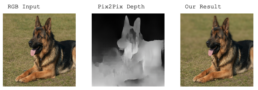
Figure 1: Demonstration of our adapted version of Pix2Pix. Notice the blur of the grass.
We implemented and adapted Pix2Pix which converts RGB data to a depth map. By using a depth map, we can generate artificial blur which allows phones to artificially replicate a camera with lower DoF. A depth map is a 1 channel output where the brighter the pixel, the closer it is to the camera.
Methods & Analysis
In this report we are required to compare and discuss the strengths and weaknesses of four different approaches. These are the image outputs which will be referred to a lot in this section.
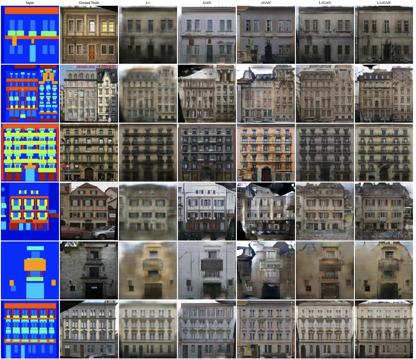
Figure 2: Output of facades comparing all four approaches. (Isola et al., 2018)
Method 1: CNNs
Classical approaches use CNNs to generate images from paired inputs. CNNs attempt to minimize a loss function: a function which quantifies how well the model is doing. Designing effective loss functions for this is difficult as it requires a lot of guesswork (Isola et al., 2018). For example, using Euclidean losses such as L1 or L2 yield blurry results due to them only being able to minimize only low frequency correctness (big details).
\[\mathcal{L}_{L1} (G) = \mathbb E_{x, y, z}[||y-G(x,z)||_{1}]\]Figure 3: Loss function of a Standard CNN
From the output samples that are shown above, we can see that CNNs produce very blurry pictures that do not look realistic at all. When given the task of recreating building facades, it generates windows and the correct colors for the buildings and even roofs (2nd figure) but cannot generate convincing wall textures (3rd figure). This is because the L1 function is too naive to be able to determine fine details such as textures. The advantages of CNN include that it is much more simpler to code and interpret the features that it learns. Additionally, it is much faster and efficient than the next methods, however it falls short in terms of performance.
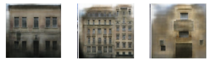
Figure 4: Samples of images created using L1 loss (CNN)
Method 2: GANs
We explore GANs as they can determine an adaptive loss function instead of using a naive, human designed one. Generative Adversarial Networks (GAN) are comprised of two models, a generator and a discriminator. The generator $G$ uses a CNN model which we will cover to create a fake image given the feature input $x$ and a random Gaussian noise $z$. It attempts to minimize the loss of the entire GAN.
The second part of the GAN is the discriminator. The goal of the discriminator is to determine whether the image is generated by the generator or is a real image. The discriminator is given both real sample images as well as fake samples created by the generator, and the discriminator’s goal is to determine whether they are real or fake. The objective of the generator is to trick the discriminator into thinking that its sample is real.
Given the real ground truth image $D(y)$, the discriminator will attempt to maximize this equation, which is derived from binary cross entropy loss.
\[\mathbb E_{y}[log D(y)]\]Conversely, the discriminator could also be fed the output of the generator $D(G(x,z))$.
\[\mathbb E_{x,z}[log(1-D(G(x,z)))]\]Summing both terms of the discriminator loss given both scenarios, we get the loss function of a traditional, unconditional GAN. The generator attempts to minimize the loss of the entire GAN hence $\min\limits_{G}$ and the discriminator attempts to maximize it hence $\max\limits_{D}$.
\[\min\limits_{G} \max\limits_{D} \mathcal{L}_{GAN}(G, D) = \mathbb E_{y}[log D(y)] + \mathbb E_{x, z}[log(1 - D(G(x, z)))]\]Loss function of a traditional GAN
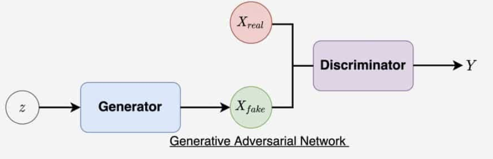
Figure 5: Diagram of a GAN. (Sharma, 2021)
GANs are efficient at reducing high frequency noise (Isola et al., 2018), which allows it to closely mimic textures and small details. This is seen in the figure as a highly detailed image, but we can see how lighting is not fully realistic. Lighting such as sunlight is therefore most likely determined by low frequency correctness as the whole image is affected by the same lighting conditions. Additionally, other parts sometimes are occluded or misshaped (look at the roofs or Xcorners of these images).
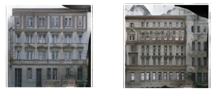
Figure 6: Samples of images created using traditional GAN
Method 3: Conditional GANs
Conditional GANs build on the concept of regular GANs. We utilized paired data meaning that each feature $x$ has a corresponding label $y$ to it. The discriminator in a cGAN can “see” this feature alongside the ground truth and make a more accurate evaluation as of a result. This means that given real samples, the discriminator is also fed the input features $D(x,y)$ and given fake samples created by the generator it is also fed the input features $D(x, G(x, z))$. This changes the loss function to this.
\[\min\limits_{G} \max\limits_{D} \mathcal{L}_{cGAN} (G, D) = \mathbb E_{x, y}[log D(x, y)] + \mathbb E_{x, z}[log(1 - D(x, G(x, z)))]\]Loss function of a conditional GAN (cGAN)
Additionally, it does not use Gaussian noise as $z$ unlike traditional GANs as experiments showed that it was ineffective (Isola et al., 2018). Instead, noise in introduced in the dropout instead.
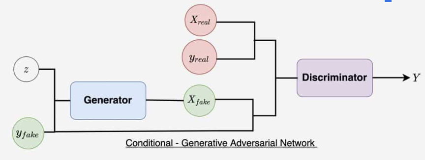
Figure 7: Diagram of a Conditional GAN. (Sharma, 2021)
By using paired data, Isola et al., (2018) claims that it learns a structured loss which penalizes the joint configuration of the output. The cGAN is more aware of modifying and recreating image styles (Redford et. al., 2016) Observing the output, it is similar to the GAN’s in which it can replicate fine details but sometimes hallucinates on other parts of the building.
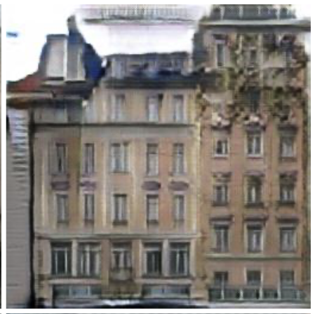
Figure 7: Samples of images created using Conditional GAN
Method 4: Pix2Pix Method
Pix2Pix combines both approaches of L1 loss (CNN-like) and cGAN loss. This is, in a sense, the “best of both worlds” as the L1 focuses on low frequency correctness such as lighting and we can choose a discriminator which emphasizes high frequency correctness. If you look at the results of the images generated by the combination of these (L1cGAN), we observe a much greater detail. They are summed up in this example. We will talk about this in more detail in the next section.
\[G^{*}=\arg\min\limits_{G} \max\limits_{D} \mathcal{L}_{cGAN} (G, D) + \lambda\mathcal{L}_{L1} (G)\]This provides the most realistic images as you can see here. It provides more accurate lighting compared to L1, GAN and cGANs. It still suffers from the corner problems but in the end it yields a much more realistic result. We will discuss the implementation and performance of these models in the next section.
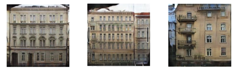
Figure 7: Samples of images created using L1 + cGAN (Pix2Pix)
Performance
The metrics determining the performance of Pix2Pix by giving the images to humans (Turkers). When converted a map (Semantic Segmentation) styled image to a photo, only 0.8% of Turkers thought it was real using method 1 (CNN). Method 4 (L1cGAN) clearly outperforms this with 18.9% but it is still not quite fully there yet.
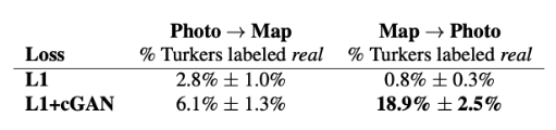
Figure 8: Performance of method 1 L1 versus method 4 L1+cGAN
When compared to the ground truth using pixel by pixel Lab values, we can see that method 4 (L1cGAN) outperforms all other methods due to its superior model as discussed.
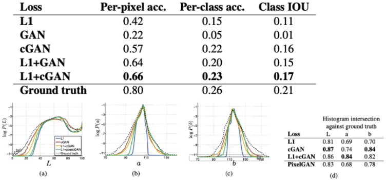
Figure 9: Comparison of histogram of images generated by all methods
Implementation
We implemented Pix2Pix (Isola et al., 2018) which originally was an Image-to-Image translation which utilizes a Conditional Generative Adversarial Network (cGAN) to produce results from paired data, meaning that each feature $x$ has a corresponding label $y$ to it. Pix2Pix’s objective is to take the feature of the paired data and generate a label of it, which is typically in a different style. For example, sometimes it is given a semantic segmentation representation as a feature and labels of the original image. It’s task is to replicate the original image through training.
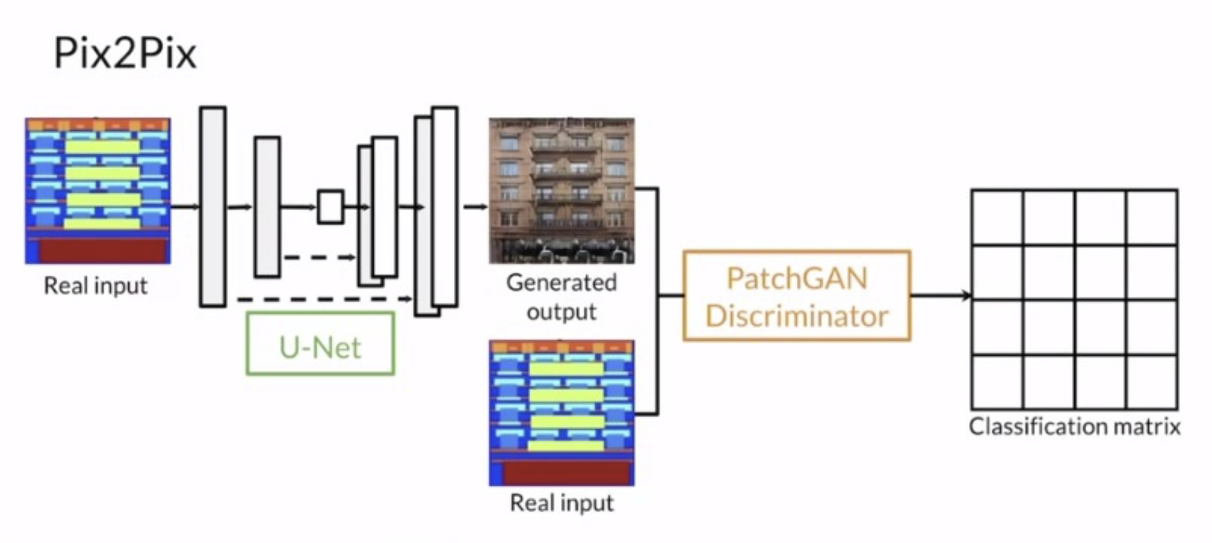
Figure 10: Architecture of Pix2Pix model. (Haiku Tech Center, 2020)
We input RGB images as a features and depth map as the paired labels. In this way, we hoped it would train based on that data and produce a realistic output, styled in the same way as other methods.
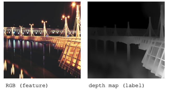
Figure 11: A sample pair of data (feature and label) we used in training.
Generator: U-Net
It uses U-Net as generator (Ronneberger et. al, 2015). It was chosen because of its proven track record and high performance. It involves downsampling an image using max pooling (left side) into a much lower resolution but higher channel representation. This means that it can remember a lot of context whilst also attempting to abstract away insignificant details. It is then upsampled using “2x2 convolution (’up-convolution’) that halves the number of feature channels” followed by 3x3 convolutions with ReLUs (Ronneberger et. al, 2015).
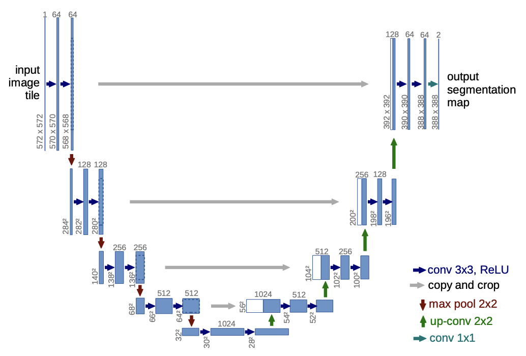
Figure 12: Diagram of U-net architecture (Ronneberger et. al, 2015)
Defining the generator in TensorFlow (TensorFlow, 2019)
def Generator():
  inputs = tf.keras.layers.Input(shape=[256, 256, 3])

  down_stack = [
    downsample(64, 4, apply_batchnorm=False),  # (batch_size, 128, 128, 64)
    downsample(128, 4),  # (batch_size, 64, 64, 128)
    downsample(256, 4),  # (batch_size, 32, 32, 256)
    downsample(512, 4),  # (batch_size, 16, 16, 512)
    downsample(512, 4),  # (batch_size, 8, 8, 512)
    downsample(512, 4),  # (batch_size, 4, 4, 512)
    downsample(512, 4),  # (batch_size, 2, 2, 512)
    downsample(512, 4),  # (batch_size, 1, 1, 512)
  ]

  up_stack = [
    upsample(512, 4, apply_dropout=True),  # (batch_size, 2, 2, 1024)
    upsample(512, 4, apply_dropout=True),  # (batch_size, 4, 4, 1024)
    upsample(512, 4, apply_dropout=True),  # (batch_size, 8, 8, 1024)
    upsample(512, 4),  # (batch_size, 16, 16, 1024)
    upsample(256, 4),  # (batch_size, 32, 32, 512)
    upsample(128, 4),  # (batch_size, 64, 64, 256)
    upsample(64, 4),  # (batch_size, 128, 128, 128)
  ]

  initializer = tf.random_normal_initializer(0., 0.02)
  last = tf.keras.layers.Conv2DTranspose(OUTPUT_CHANNELS, 4,
                                         strides=2,
                                         padding='same',
                                         kernel_initializer=initializer,
                                         activation='tanh')  # (batch_size, 256, 256, 3)

  x = inputs

  # Downsampling through the model
  skips = []
  for down in down_stack:
    x = down(x)
    skips.append(x)

  skips = reversed(skips[:-1])

  # Upsampling and establishing the skip connections
  for up, skip in zip(up_stack, skips):
    x = up(x)
    x = tf.keras.layers.Concatenate()([x, skip])

  x = last(x)

  return tf.keras.Model(inputs=inputs, outputs=x)
and also the generator loss (TensorFlow, 2019), This is equivalent to the equation we covered in method 4 (L1cGAN)
LAMBDA = 100
loss_object = tf.keras.losses.BinaryCrossentropy(from_logits=True)
def generator_loss(disc_generated_output, gen_output, target):
  gan_loss = loss_object(tf.ones_like(disc_generated_output), disc_generated_output)

  # Mean absolute error
  l1_loss = tf.reduce_mean(tf.abs(target - gen_output))

  total_gen_loss = gan_loss + (LAMBDA * l1_loss)

  return total_gen_loss, gan_loss, l1_loss
Discriminator: PatchGAN
PatchGAN (Li, Wand, 2016) was chosen by the authors of Pix2Pix as the discriminator. It utilizes Markovian patches, a process which mainly focuses high frequency details and therefore excels at synthesizing stylized textures such as in this example. Isola et. al (2018) claims that PatchGAN “is effective on a wider range of problems” and “can be understood as a form of texture/style loss”. We do not need the discriminator to worry too much about the low-frequency correctness as we described in the previous section that L1 loss will account for that.
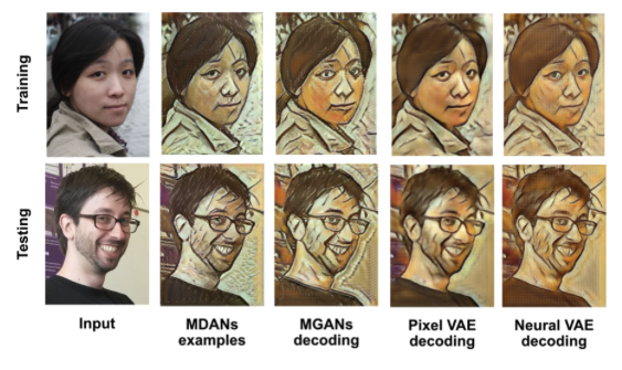
Figure 13: Results of PatchGAN (Li, Wand, 2016)
We define the discriminator using TensorFlow (TensorFlow, 2019)
def Discriminator():
  initializer = tf.random_normal_initializer(0., 0.02)

  inp = tf.keras.layers.Input(shape=[256, 256, 3], name='input_image')
  tar = tf.keras.layers.Input(shape=[256, 256, 3], name='target_image')
  x = tf.keras.layers.concatenate([inp, tar])  # (batch_size, 256, 256, channels*2)

  down1 = downsample(64, 4, False)(x)  # (batch_size, 128, 128, 64)
  down2 = downsample(128, 4)(down1)  # (batch_size, 64, 64, 128)
  down3 = downsample(256, 4)(down2)  # (batch_size, 32, 32, 256)

  zero_pad1 = tf.keras.layers.ZeroPadding2D()(down3)  # (batch_size, 34, 34, 256)
  conv = tf.keras.layers.Conv2D(512, 4, strides=1,
                                kernel_initializer=initializer,
                                use_bias=False)(zero_pad1)  # (batch_size, 31, 31, 512)

  batchnorm1 = tf.keras.layers.BatchNormalization()(conv)
  leaky_relu = tf.keras.layers.LeakyReLU()(batchnorm1)
  zero_pad2 = tf.keras.layers.ZeroPadding2D()(leaky_relu)  # (batch_size, 33, 33, 512)

  last = tf.keras.layers.Conv2D(1, 4, strides=1,
                                kernel_initializer=initializer)(zero_pad2)  # (batch_size, 30, 30, 1)

  return tf.keras.Model(inputs=[inp, tar], outputs=last)
Visualization of the discriminator
discriminator = Discriminator()
tf.keras.utils.plot_model(discriminator, show_shapes=True, dpi=64)
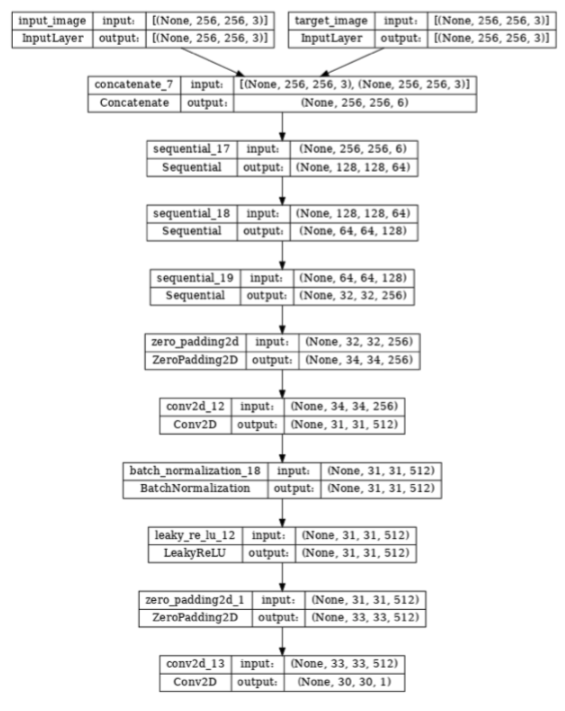
Figure 14: Architecture of PatchGAN
We define the discriminator loss (TensorFlow, 2019)
def discriminator_loss(disc_real_output, disc_generated_output):
  real_loss = loss_object(tf.ones_like(disc_real_output), disc_real_output)

  generated_loss = loss_object(tf.zeros_like(disc_generated_output), disc_generated_output)

  total_disc_loss = real_loss + generated_loss

  return total_disc_loss
Database
We compared a multitude of datasets in this project. In the end we picked the DIML Indoor dataset to train the model on due to its realistic scenarios of data covering indoor scenes. Additionally, it boasts accurate depth map ground truths because these images were captured using a Kinect v2 or a Zed stereo camera. It is very large and has a lot of variations which is optimal in preventing overfitting.
The code to download the dataset can be seen here. It was uploaded to Google Colab and then downloaded into the Colab file as such. (TensorFlow, 2019)
def load(image_file):
  # Read and decode an image file to a uint8 tensor
  image = tf.io.read_file(image_file)
  image = tf.io.decode_jpeg(image)

  # Split each image tensor into two tensors:
  # - one with a real building facade image
  # - one with an architecture label image
  w = tf.shape(image)[1]
  w = w // 2
  input_image = image[:, w:, :]
  real_image = image[:, :w, :]

  # Convert both images to float32 tensors
  input_image = tf.cast(input_image, tf.float32)
  real_image = tf.cast(real_image, tf.float32)

  return input_image, real_image

def load_image_train(image_file):
input_image, real_image = load(image_file)
input_image, real_image = random_jitter(input_image, real_image)
input_image, real_image = normalize(input_image, real_image)

return input_image, real_image

def load_image_test(image_file):
  input_image, real_image = load(image_file)
  input_image, real_image = resize(input_image, real_image,
                                   IMG_HEIGHT, IMG_WIDTH)
  input_image, real_image = normalize(input_image, real_image)

  return input_image, real_image

train_dataset = tf.data.Dataset.list_files(str(PATH / 'train/*.jpg'))
train_dataset = train_dataset.map(load_image_train,
                                  num_parallel_calls=tf.data.AUTOTUNE)
train_dataset = train_dataset.shuffle(BUFFER_SIZE)
train_dataset = train_dataset.batch(BATCH_SIZE)

try:
  test_dataset = tf.data.Dataset.list_files(str(PATH / 'test/*.jpg'))
except tf.errors.InvalidArgumentError:
  test_dataset = tf.data.Dataset.list_files(str(PATH / 'val/*.jpg'))
test_dataset = test_dataset.map(load_image_test)
test_dataset = test_dataset.batch(BATCH_SIZE)
Training
We trained the model on 10 epochs and experimented with various different batch sizes. We stopped training after we noticed that the loss started converging. We settled on a batch size of 1 and a training size of 1610 images. The test set was split at around 20% of the data so at 320 images. We determined that this was large enough to not cause overfitting as our training and test loss were fairly similar.
This is the training code (TensorFlow, 2019)
@tf.function
def train_step(input_image, target, step):
  with tf.GradientTape() as gen_tape, tf.GradientTape() as disc_tape:
    gen_output = generator(input_image, training=True)

    disc_real_output = discriminator([input_image, target], training=True)
    disc_generated_output = discriminator([input_image, gen_output], training=True)

    gen_total_loss, gen_gan_loss, gen_l1_loss = generator_loss(disc_generated_output, gen_output, target)
    disc_loss = discriminator_loss(disc_real_output, disc_generated_output)

  generator_gradients = gen_tape.gradient(gen_total_loss,
                                          generator.trainable_variables)
  discriminator_gradients = disc_tape.gradient(disc_loss,
                                               discriminator.trainable_variables)

  generator_optimizer.apply_gradients(zip(generator_gradients,
                                          generator.trainable_variables))
  discriminator_optimizer.apply_gradients(zip(discriminator_gradients,
                                              discriminator.trainable_variables))

  with summary_writer.as_default():
    tf.summary.scalar('gen_total_loss', gen_total_loss, step=step//1000)
    tf.summary.scalar('gen_gan_loss', gen_gan_loss, step=step//1000)
    tf.summary.scalar('gen_l1_loss', gen_l1_loss, step=step//1000)
    tf.summary.scalar('disc_loss', disc_loss, step=step//1000)

def fit(train_ds, test_ds, steps):
  example_input, example_target = next(iter(test_ds.take(1)))
  start = time.time()

  for step, (input_image, target) in train_ds.repeat().take(steps).enumerate():
    if (step) % 1000 == 0:
      display.clear_output(wait=True)

      if step != 0:
        print(f'Time taken for 1000 steps: {time.time()-start:.2f} sec\n')

      start = time.time()

      generate_images(generator, example_input, example_target)
      print(f"Step: {step//1000}k")

    train_step(input_image, target, step)

    # Training step
    if (step+1) % 10 == 0:
      print('.', end='', flush=True)

    # Save (checkpoint) the model every 5k steps
    if (step + 1) % 5000 == 0:
      checkpoint.save(file_prefix=checkpoint_prefix)

fit(train_dataset, test_dataset, steps=40000)

# Run the trained model on a few examples from the test set
for inp, tar in test_dataset.take(5):
  generate_images(generator, inp, tar)
Post-Processing
We wrote a blurring method designed to convert the depth map into bokeh blur from display. This is the code for that.
import cv2
import numpy as np
import requests
from tqdm import tqdm
import warnings
import matplotlib as mpl
import matplotlib.pyplot as plt

warnings.filterwarnings("ignore")

# how many images are there?
n_images = 10
img_data = np.empty([n_images, 3, 256, 256, 3])

def blur():
  for n in range(n_images):
    # test image loading
    test=True
    print('test mode ON')
    print('loading image...')
    img = cv2.imread("rgb" + str(n) + ".png", cv2.IMREAD_COLOR)
    print(img.shape)
    img_data[n, 0] = img
    #cv2.imwrite('img_input.png', img)
    print('image loaded')

    # make blur map
    height = img.shape[0]
    width = img.shape[1]
    blur_map = cv2.imread("d" + str(n) + ".png", cv2.IMREAD_COLOR)
    img_data[n, 1] = blur_map
    blur_scale = 30

    for c in range(blur_map.shape[2]):
      for x in tqdm(range(width)):
          for y in range(height):
            blur_map[x, y, c] = min(max((150 - blur_map[x, y, c]) / blur_scale, 0), 254)
    cv2.imwrite('blurmap.png', blur_map );

    # very inefficient blur algorithm!!!
    img_blur = np.copy(img)
    for c in range(img.shape[2]):
      for x in tqdm(range(width)):
          for y in range(height):
              kernel_size = int(blur_map[y, x, 0])

              # no blur applied, then just skip
              if kernel_size == 0:
                  img_blur[y, x, c] = img[y, x, c]
                  continue

              kernel = cv2.getStructuringElement(cv2.MORPH_ELLIPSE, (kernel_size, kernel_size))
              cut = img[
                  max(0, y - kernel_size):min(height, y + kernel_size),
                  max(0, x - kernel_size):min(width, x + kernel_size),
                  c
              ]

              if cut.shape == kernel.shape:
                  cut = (cut * kernel).mean()
              else:
                  cut = cut.mean()

              img_blur[y, x, c] = cut
    img_data[n, 2] = img_blur
    cv2.imwrite('output' + str(n) + '.png', img_blur);
    print('done')

blur()
Results
We fed some things into the data and wrote code to apply a bokeh blur to where the depth map is lightest. These are some curated samples from our test set.
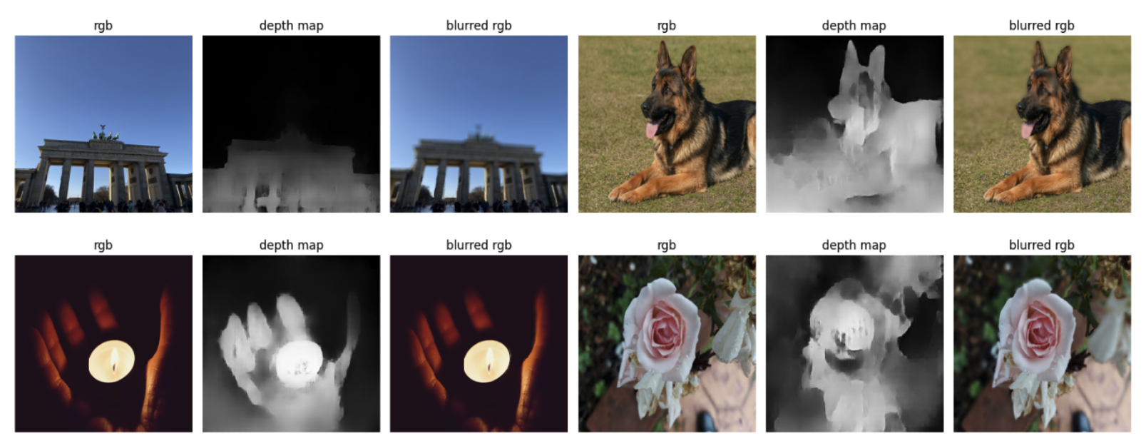
Figure 15: Our results
Discussion
We can see that it is non-optimal in some scenarios and it still struggles to pick out the edges in some photos. This may be due to us using a test set being significantly different to the training set. The training set (DIML indoor) is only comprised of indoor scenes and less of photographic subjects such as in the test data. This therefore performs worse and misrepresents objects. Look at the dogs left eye or the rose petal that is incorrectly labeled as being far away. This results in blurring of the wrong parts and inaccurate results.
Overall, this is a semi effectively solution for implementing monocular depth estimation. With a larger database with more variations and longer training times, we may be able to go closer to hardware-like similarities. This tool can be purposed other uses such as SLaM and robotics as well.
Works Cited
- Haiku Tech Center. (2020). Pix2Pix GAN Architecture For Image. https://www.haikutechcenter.com/2020/10/pix2pix-gan-architecture-for-image-to.html
- Isola P., Et Al. (2018) Image-to-Image Translation with Conditional Adversarial Networks. https://arxiv.org/pdf/1611.07004.pdf
- Li C., Wand M., (2016) Precomputed real-time texture synthesis with markovian generative adversarial networks. ECCV. https://arxiv.org/pdf/1604.04382.pdf
- Radford A., Et Al. (2016) Unsupervised Representation Learning with Deep Convolutional Generative Adversarial Networks. https://arxiv.org/pdf/1511.06434.pdf
- Ronneberger O., Et Al. (2015). U-net: Convolutional networks for biomedical image segmentation. MIC CAI. https://arxiv.org/pdf/1505.04597.pdf
- Sharma A. (2021) Conditional GAN cGAN in Pytorch and TF. https://learnopencv.com/conditional-gan-cgan-in-pytorch-and-tensorflow/
- TensorFlow. (2019) pix2pix https://www.tensorflow.org/tutorials/generative/pix2pix