In this blog article, we’ll delve into CLIP(Contrastive Language-Image Pre-training), focusing primarily on its application in zero-shot classification. Unlike examining a pre-trained version, we will embark on training CLIP ourselves, crafting the core components of the model and employing a distinct, smaller dataset for training purposes. We’ll also introduce custom loss functions and dissect specific elements of CLIP, such as its contrastive loss mechanism. This article aims to dissect the architecture and its implications, making minor adjustments to better grasp what drives its effectiveness.

• Table of Contents
  • Introduction to Zero-Shot Learning, Previous Methods, and Their Shortfalls
  • Introduction to CLIP
  • Results of CLIP
  • Experimentation
    • Triplet loss
    • Queue addition (Personal Implementation!)
    • Results
  • Conclusion
  • An output of the model, enjoy!
  • Acknowledgments
  • References

Table of Contents

Introduction to Zero-Shot Learning, Previous Methods, and Their Shortfalls

What exactly is zero-shot classification? Zero-shot classification models have the ability to classify data that hasn’t been seen during training. Consider a model trained to differentiate all mammals from Africa; if it can classify mammals from other parts of the world without being trained on those specific animals, then it possesses zero-shot capabilities for this newly extended class set. Furthermore, a model is said to have n-shot classification capabilities if it maintains a certain accuracy on unseen classes, after being trained with n instances per class.

The essence here is the attempt to generalize models to learn from the relationships between classes to predict the characteristics of new classes. Previously, conventional computer vision was rooted in a fixed-class framework where classification was limited to a predefined set of classes, and accuracy was derived from this constraint. Now, machine learning scientists aim to generalize these potent methods to adeptly classify unseen data as well. So, what’s the hitch with this approach? The hitch lies in the computational expense of training models on unseen classes and the vast number of classes that potentially exist. The plethora of possible image classes makes it exceedingly challenging to train a model to recognize all these classes. Nevertheless, if our models can learn more general and intrinsic image representations, they’ll be better equipped to extend their knowledge to unseen data classes.

So, how can we achieve this? How can we develop models that can learn more general patterns, models that can adapt to unseen class sets? Let’s examine some previous research addressing this issue. In Attribute-Based Classification for Zero-Shot Visual Object Categorization, the author attempts to classify images zero-shot by mapping an image to a specific set of attributes and then using those attributes as classification weights for a class. Essentially, they’re constructing an attribute classifier and leveraging it to classify unseen data. This approach is feasible as unseen data may share attributes with the pre-training dataset. Although innovative at the time, this technique’s limitation is the prerequisite to label unseen classes by their attributes before classification, plus, unseen classes might have quite disparate sets of attributes, demanding more representational power.

Subsequent papers like Zero-Shot Learning by Convex Combination of Semantic Embeddings, DeViSE: A Deep Visual-Semantic Embedding Model, and Zero-Shot Learning with Semantic Output Codes refine this concept by aligning images with a set of embedding representations. The elegance of this methodology lies in the fact that embeddings can encapsulate a rich representation of the image and its semantic meaning, facilitating a seamless extrapolation to unseen data, and containing much more information than mere attributes. Specifically, the DeViSE method introduces a novel way of pairing images and their corresponding semantic representations using a similarity score, enabling the image to emit a continuous embedding representation for richer interpretations. A critical aspect of zero-shot classification here is comparing the image’s outputted embedding with the label’s embedding, where the highest similarity dictates the classification. This approach achieved impressive results in certain zero-shot classification categories.

As often happens, Google initiated this line of inquiry, which OpenAI then expanded upon, adding its unique contributions and scaling the concept significantly. This model was henceforth known as CLIP.

Introduction to CLIP

So what exactly is CLIP? The model was originally introduced in the paper Learning Transferable Visual Models From Natural Language Supervision, as having two main parts, a powerful image and a text encoder. The essence of CLIP lies in taking two powerful encoders mapping their output latent space representation and aligning this output to a multimodal embedding space. Effectively theta re trying to create a multimodal space that is defined by some distance metric, in the case of CLIP the distance metric is the dot product(cosine similarity) between the two mapped embeddings. The closer teh embeddings the higher their corresponding similarity score will be. Isn’t that amazing?

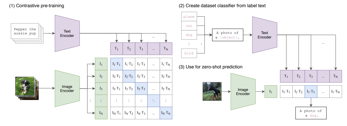
Fig 1. Overview of the CLIP Architecture. This image was taken form the original paper cited in the references. As the figure above shows CLIP has two main parts the text encoder and image encoder, the text encoder outputs a batch of text embedding and the image a batch of image embeddings, this image and text embeddings are then mapped using a linear transformation to a common embedding space. After which we take the dot product, and calculate the loss(details later). During inference for zero shot classification the text is generated by using some predefined set of text, for example if we wanted to classify dogs and cats. The text code be “This is an image of a cat”, “This is a photo of a cat”, or even “Here lies a cat, a majestic animal, man’s favorite pet”(for the cat lovers out there). The point is that the text can be any text that describes the image in fact the authors of the paper actually had some studies on the effect of prompt engineering(see paper for details).

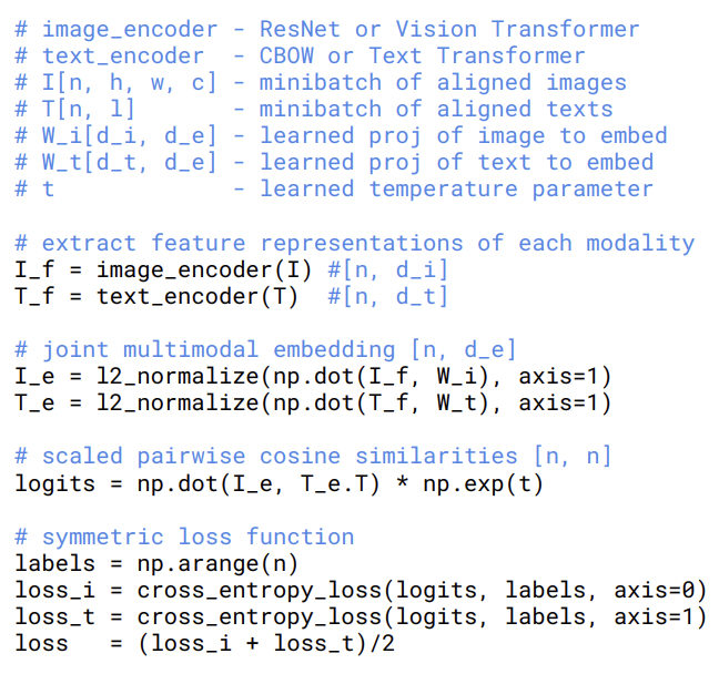
Fig 2. Overview of the CLIP Loss. This image was taken form the original paper. The figure above illustrates the core implementation and loss function of CLIP. CLIP uses a Multi Class N-pair loss. Essentially what happens is for every batch, every possible pair of image and text embeddings is generated after which the cross entropy loss for the image encoder and text encoder is taken seperately. Then the loss is added together. The key here is that the loss is calculated by looking at the dot product values as probabilities(in pytorch softmax is in the cross entropy class). So for an image encoder the loss is calculated by how well it’s given image is correlated with the correct text, while for text encoder how well the generated text is closely correlated with the image

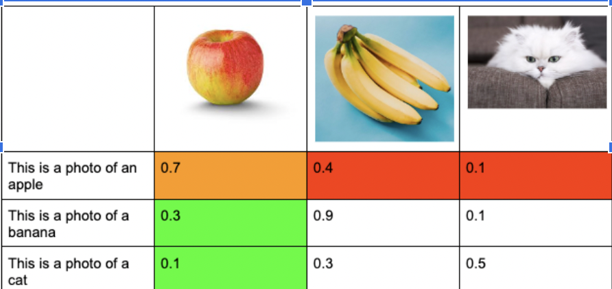
Fig 3. This figure is an example of the loss calculations for CLIP. The values are the logits which will be inputted into cross entropy layer. The green represents the logits for the image encoder, the image encoder wants to maximize the the probability of getting a high similarity score with the correct text embedding, while the text encoder wants to do the same for it’s text embedding(red part is a part of the text encoder’s loss)

Some key points before we move on. In the original paper the authors stated that they used a batch size of around 32000(gigantic). The primary purpose was for computational effeciency. Additionally the authors used different models for their image encoders, such as Resnet 50 and VIT large. The text encoder was a transformer. They used a dataset of 400 million image caption paris scrapped of the internet. The question now becomes how effective is this model. Lets analyze some of the results

Results of CLIP

CLIP perform very well in a zero shot setting the following figures will explain look at some results.

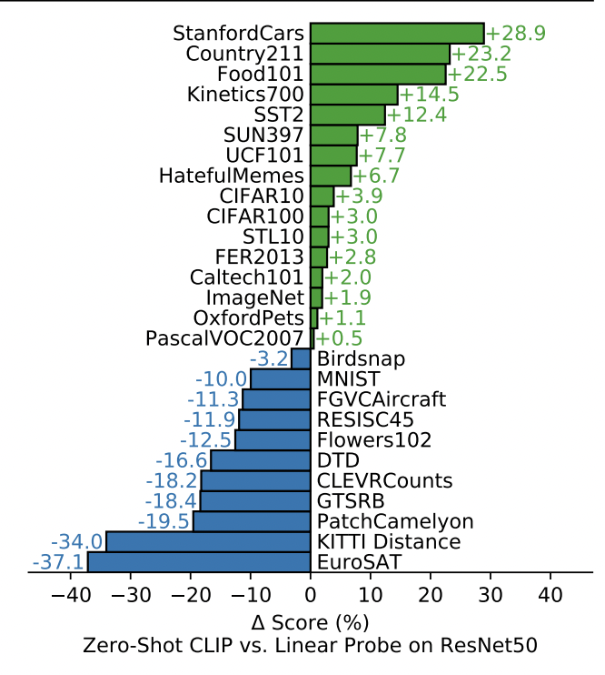
Figure 4 shows another image taken from the original paper. It contains many different datasets and the accuracy difference between CLIP and Resnet50 with a linear probe. Remarkably CLIP performs better!

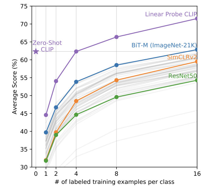
Figure 5 shows another image taken from the original paper. In this case different models were trained and the accuracy after n training instances per example was taken. CLIP performs better significantly better zero shot even compared to 15 shot BiT-M!

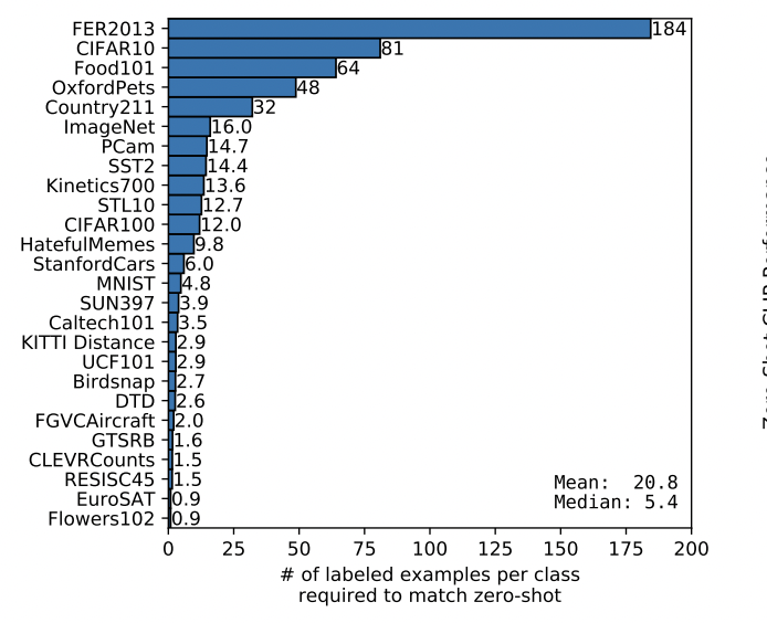
Figure 6 shows another image taken from the original paper. It shows the average and median number of training instances required per class to surpass CLIP zero shot. When one sees 12 for CIFAR100 it may seem small, but indeed 12 images per class is actually 1200 images all together

The results show that CLIP does perform well in a Zero shot setting. So well in fact that it outperforms that models need to learn from quite a number of images before they can match CLIP. Let us dive deeper into this intriguing model and breakdown some of the implementation details.

Experimentation

The goal is to implement the paper from scratch to get a better understanding of the underlying architecture. In my case I implemented a version of CLIP based on my hardware limitations( NVIDIA please help me out, I can’t keep using money on Colab). For my image encoder I used a pretrained Resnet model, while for my text encoder I used a pretrained GPT2 model. I had a batch size of 64. For my image encoder I mapped the final layer before the linear layer to a embedding representation by average pooling the feature maps. I trained it for 5 epochs(as opposed to 30 in the research paper), and had about a 1 million images in the training dataset. Due to time constraints I focused on CIFAR 10 as a zero shot setting for CLIP. Additionally I used ADAMW for my optimizer, and also occasionally decreased the learning rate using a scheduler. Here is a snippet of my CORE CLIP implementation.

This here is the class implementation for my image encoder, as said before it simply takes the adaptive average pool of the feature maps and then outputs that as the image embedding.

class ImageEncoder(nn.Module):
    def __init__(self, mode='finetune'):
        super().__init__()
        weights = ResNet50_Weights.IMAGENET1K_V1
        self.resnet = resnet50(weights=weights)
        
        self.resnet = nn.Sequential(*list(self.resnet.children())[:-2])
        self.adaptive_pool = nn.AdaptiveAvgPool2d((1))

    def forward(self, x):
        x = self.resnet(x)
        x = self.adaptive_pool(x)
        x = torch.reshape(x, (x.shape[0], x.shape[1]))
        return x

    def to(self, device):
        super().to(device)
        return self

This is my text encoder class, this simply uses a GPT 2 model with pretrained weights for text embedding generation, I take the last hidden state as the text embedding.

class TextEncoder(nn.Module):

    def __init__(self):
        super().__init__()

        self.tokenizer = GPT2Tokenizer.from_pretrained('openai-community/gpt2')
        self.model = GPT2Model.from_pretrained('openai-community/gpt2')
        self.tokenizer.pad_token = self.tokenizer.eos_token
    def forward(self, texts):
        inputs = self.tokenizer(texts, return_tensors='pt', padding=True, truncation=True)
        inputs = {k: v.to(device) for k, v in inputs.items()}

        outputs = self.model(**inputs)
        return outputs.last_hidden_state[:, -1, :]

    def to(self, device):
        self.model = self.model.to(device)
        return self

This is the forward method for CLIP module. Essentially it takes the embedding from image and text encoders and then puts them through a linear transformation. After which it normalizes the tensors for use later on(similarity scores require normalized vectors).

def forward(self, image, text):(FOR CLIP MODEL)
    image_embedding = self.image_encoder(image)
    text_embedding = self.text_encoder(text)
    image_embedding = self.image_projection(image_embedding)
    image_embedding = self.image_layer1(image_embedding)
    
    text_embedding = self.text_projection(text_embedding)
    text_embedding = self.text_layer1(text_embedding)
    
    # Normalize embeddings
    image_embedding = F.normalize(image_embedding, p=2, dim=-1)
    text_embedding = F.normalize(text_embedding, p=2, dim=-1)
    # decoded_image = self.image_decoder(image_embedding)
    return image_embedding, text_embedding

This is the core part of the loss calculation, I take the normalized embeddings and take the dot product, after which I take teh respective image and text encoder loss and backpropogate using the sum of the two.

#Labels for each entry
labels = torch.arange(img_emb.shape[0], device=device)
logits_img_text = torch.matmul(img_emb, text_mat.t()) * 2
logits_text_img = torch.matmul(text_emb, img_mat.t()) * 2
#Calculate losss
img_text_loss = F.cross_entropy(logits_img_text, labels) 
text_img_loss = F.cross_entropy(logits_text_img, labels)
final_loss = (img_text_loss + text_img_loss)/2
final_loss.backward()
optimizer.step()

And so I trained my model, and prayed some good grace. Surprisingly the model actually performed decent on CIFAR 10, it got 45.2% accuracy! On CIFAR 100 it didn’t do as well but this was expected, it had an accuracy of 13.6%.

During this experience one question became very evident. How would does the loss function affect CLIP, would using another loss say Triplet loss be more effective? Also given that CLIP uses such a large batch size in the original paper what are some ways one can simulate this without having any major memory impacts?

Triplet loss

Triplet loss, is another interesting loss functions used to teach a model negative and positive representations of a class. As teh name suggest it is based on three important parts, the anchor, negative examples, positive examples. The anchor is the object in question, in our case the image tor text that will be matched to their corresponding pairs. While the negative and positive examples, are parts of the dataset that are different to the anchor and a positive match. For the image encoder the parts of the mapped text embedding pair is the positive example, while the other non paired embeddings are negative.
The implementation is illustrated below

img_text_similarity = torch.matmul(img_emb, text_emb.t()).diag()
n = img_emb.shape[0]
original_list = list(range(n))
shifted_list = original_list[1:] + [original_list[0]]
shuffled_image = img_emb[shifted_list]
shuffled_text = text_emb[shifted_list]
neg_sim_img = torch.matmul(img_emb, shuffled_text.t()).diag()
neg_sim_text = torch.matmul(text_emb,shuffled_image.t()).diag()
img_loss = torch.clamp(margin + neg_sim_img - img_text_similarity, min=0)
text_loss = torch.clamp(margin + neg_sim_text - img_text_similarity, min=0)      
final_loss = (img_loss.mean() + text_loss.mean())/2

All I am doing here is making an anchor(ie img_emb, text_emb), shuffling the batch in the batch dimensions and then taking forming matrix multiplication on the original unshuffled tensor and the shuffled tensor(positive and negative examples). Interestingly triplet loss can be seen as an example of our previous loss. Imagine having just two pairs previously then the dot product of the incorrect pairs can be seen as a negative example and the correct pairs as a positive example. If we don’t include the second pair, we have a form of Triplet loss.

Queue addition (Personal Implementation!)

One major problem that is evident from the paper is the requirment of using large batch sizes for training. This was needed at the time for effeciency reasons. Additionally it seems that a larger batch size would lead to better contrastive learning capabilities as embedding would have more positive and negative comparisons to learn from in a given batch. So I thought of using a some sort of queue that I can randomly sample from in a given batch, to extend the batch size. This way I could bypass the memory requirements for large batch size by just storing the embeddings in queue and taking out iteratively popping the queue to decrease the size.

Additionally I thought that due to the nature of storing embedding in a queue, the generated embeddings would become more robust. This is similar to the idea proposed on the research paper titled Momentum Contrast for Unsupervised Visual Representation Learning. While the purpose of the researchers was different, they used a momentum encoder to stabilize the training of their main image encoder. The secondary encoder served as a momentum factor in helping their main encoder reach more effective embedding representations( which was the goal for this). For this part I added 30 additional embeddings to the model form the queue.

Down below is the code implementation

# Get embeddings from the model
img_emb, text_emb, img_emb_att, text_emb_att = model(inputs, labels)
embedding_queue.add_queue(img_emb.clone().detach().cpu(),text_emb.clone().detach().cpu())
saved_img_embeddings, saved_text_embeddings = embedding_queue.return_values()
extra_loss = 0
if len(saved_img_embeddings) > 0:
    new_img = torch.cat(saved_img_embeddings, dim=0).to(device)
    new_text = torch.cat(saved_text_embeddings, dim=0).to(device)
    img_mat = torch.cat([img_emb, new_img ], dim=0).to(device)     
    text_mat = torch.cat([text_emb, new_text ], dim=0).to(device)             
                       
# Labels for each entry
labels = torch.arange(img_emb.shape[0], device=device)

logits_img_text = torch.matmul(img_emb, text_mat.t()) * 2
logits_text_img = torch.matmul(text_emb, img_mat.t()) * 2

# Calculate loss
img_text_loss = F.cross_entropy(logits_img_text, labels) 
text_img_loss = F.cross_entropy(logits_text_img, labels)
final_loss = (img_text_loss + text_img_loss)/2

Results

Triplet loss had an accuracy of around 33.26% on CIFAR 100 it performed with an accuracy of 8.46. It performed reasonably well, while it is nowhere clos to Multi Class N-pair loss, given more data and larger number of epochs, this loss function seems to be able to have good results. What’s more interesting is that it only takes in to account three data instances and so serves as a sort of extreme end bound for Multi Class N-pair. The queue based approach achieved a 10.93%, 43.42% accuracy respectively. Interestingly while viewing the validation loss I saw that the queue based approach was very slow to start moving down. Additionally compared to Multi Class N-pair loss the accuracy(tested in between epochs) moved slowly as well. This can hint on the fact that the models embeddings have to be more robust during loss calculation as they are compared with additional examples as well. This can serve as a good regularization factor, but must be studied on a larger scale for accurate results.

Conclusion

This exploration of CLIP, from its foundational concepts to hands-on experimentation, reveals the model’s versatility and power in zero-shot classification. By delving into its architecture and tweaking various components, we gain a deeper understanding of what makes CLIP effective and the future directions for research in this area. To further experiment I would like to look at more zero shot settings, and increase teh dataset, batch and epoch size of my experiments. This way I can run more reliable and robust experiments.

An output of the model, enjoy!

This is an output of the model given a prompt “The big blue ocean”, kinda cool!

Acknowledgments

I would like to say a special thank you to Professor Zhou for all the help and our TA Zhizheng for helping finding good sources(like the momentum paper).

References

Radford, Alec, et al. “Learning Transferable Visual Models From Natural Language Supervision.” OpenAI, 2021. Web. 22 Mar. 2024.

Lampert, Christoph H., Hannes Nickisch, and Stefan Harmeling. “Attribute-Based Classification for Zero-Shot Visual Object Categorization.” IEEE Transactions on Pattern Analysis and Machine Intelligence, vol. 36, no. 3, 2014, pp. 453-465.

Frome, Andrea, et al. “DeViSE: A Deep Visual-Semantic Embedding Model.” Advances in Neural Information Processing Systems, 2013. Web. 22 Mar. 2024.

Akata, Zeynep, et al. “Zero-Shot Learning by Convex Combination of Semantic Embeddings.” Machine Learning Research, vol. 15, 2014, pp. 935-959.

Norouzi, Mohammad, et al. “Zero-Shot Learning with Semantic Output Codes.” Journal of Machine Learning Research, vol. 14, Feb. 2014, pp. 141-171.

He, Kaiming, et al. “Momentum Contrast for Unsupervised Visual Representation Learning.” Proceedings of the IEEE/CVF Conference on Computer Vision and Pattern Recognition (CVPR), 2020, pp. 9729-9738.