Pose Estimation
The problem of Human Pose Estimation is widely applicable in computer vision—almost any task involving human interaction could benefit from pose estimation. As such, we explore the techniques and developments in this field by discussing three works relevant and reflective of these advances.
Ever since the breakthrough success of AlexNet in 2012, computer vision has experienced a surge in innovation and progress. Across countless fields, almost any task that can incorporate computer vision has benefitted tremendously from this development. As with all computer vision problems, the performance of human pose estimation has risen to incredible heights. Given the value of recognizing and interacting with humans, understanding what human pose estimation is, and how it works, is quite important.
Introduction
Human Pose Estimation—occasionally shortened to just Pose Estimation—is the process of predicting and labeling the pose of a human body from a 2D image or video. In essence, the algorithm produces a model—the pose—of the person or people it observes. Pose is typically represented as several keypoints joined by a skeleton. These keypoints are usually joints and important facial features, however many alternatives to keypoints exist, such as contour models and volumetric models. This highlights a difficulty in covering pose estimation in its entirety: the problem is both broad enough and important enough that many variations of this problem exist. Variations include using volumetric models instead of keypoints, using 3D inputs such as Lidar maps instead of traditional image data, and even dropping the “human” part of human pose estimation and predicting the orientation of objects. In general, however, Pose estimation can be broken into two primary categories—2D estimation and 3D estimation—with the difference being that 2D estimation creates an estimated human model drawn in 2 dimensions, whereas the 3D estimation generates a 3D model representing the human. The rest of this post focuses on keypoint-predicting 2D Pose Estimation, due to a particular wealth of research dedicated to this problem, and the fact that this forms a key basis for most other pose estimation variants.
Formalization
To formalize the problem: the pose estimation model must minimize overall loss in predicting keypoint locations. Regardless of the exact loss calculation, this means the model should predict the keypoints as accurately as possible. There are two principal methods for finding these keypoints: coordinate regression and heatmap regression.
Coordinate regression is simply a regression task. Each input image is labeled with ground truth keypoint coordinates, and the loss is the distance between the predicted keypoint and the exact keypoint. Any distance calculation works, but the \(L_{2}\) norm is perhaps the most common, and is used in calculating the mean squared error: \(\text{MSE}(\mathbf{y}, \hat{\mathbf{y}}) =\frac{1}{n} \|\mathbf{y} - \hat{\mathbf{y}}\|_2^2\). Coordinate regression enjoyed greater popularity in early pose estimators. A notable factor for their gradual decrease in popularity comes from a difficulty in isolating hidden keypoints. This eventually led to the rise of heatmap regression.
Heatmap regression is more common in modern implementations, both due to its performance advantages and the growing size of datasets which support this method. Here, images are labeled with keypoint heatmaps, rather than exact coordinates. These heatmaps reflect the likelihood of a keypoint being in a particular area, which makes the task more lenient on the model, as well as representing the reality that a keypoint’s exact location is not tied to a single pixel. Just as the label coordinates were converted to heatmaps, the model must now predict heatmaps instead of coordinates. A heatmap is predicted for each keypoint, with loss usually being MSE calculated with respect to each pixel. This method is notably more robust to occluded keypoints, due to the ability of heatmaps to reflect uncertainty. This method is not flawless, however; a notable difficulty with heatmap-based methods is sub-pixel accuracy. In most heatmap-based pose estimators, input images are typically downsampled significantly, such that the resulting resolution is quite low when initial heatmap predictions are made. This means significant information lies between pixels and isn’t immediately encoded into the image. When upsampling back to the original resolution, this information may be lost, even when interpolating, leading to inaccuracies. This downsample/upsample process can’t be avoided—heatmap regression is much more computationally intensive than coordinate regression, since mean squared error is calculated for each pixel in the predicted heatmap, rather than a single coordinate pair. Despite this, heatmap regression has grown popular enough to be considered the standard method in modern pose estimation.
Evaluation Metrics
Unlike loss calculation, evaluation metrics are significantly more diverse for pose estimation. Some of the more common metrics include the following:
- Percentage of Correct Parts (PCP): A limb is considered detected if the distance between the limb’s true keypoints and the limb’s predicted keypoints is at most half the limb length.
- Percentage of Correct Keypoints (PCK): A joint is considered detected if the distance between the true keypoint and the predicted keypoint is within some fraction of the torso diameter (PCK) or some fraction of the head bone length (PCKh)
- Object Keypoint Similarity (OKS): This score is the average keypoint similarity of the predicted pose: \(\frac{\sum_i KS_i \ast \delta(v_i > 0)}{\sum_i \delta(v_i > 0)}\), \(KS_i\) is the keypoint similarity for keypoint \(i\), and \(δ(v_i > 0) = 1\) for any labeled keypoint.
- Keypoint similarity is calculated by passing \(L_{2}\) distance through an unnormalized Gaussian distribution: \(KS_i = \exp\left(-\frac{d_i^2}{2s^2 k_i^2}\right)\), where \(d\) is the \(L_{2}\) distance from the true keypoint, and \(sk_i\) is the standard deviation for the Gaussian. \(s^2\) is the segmented area of the detected person, while \(k_i\) is a constant associated with each keypoint—this constant is often manually tuned for each keypoint.
Datasets
Just as many evaluation metrics exist, even more datasets exist. Major factors in considering what dataset to use include the types of poses, if the dataset is single-person or multi-person—an example of a multi person image is in the bottom right—if the data is images or videos, how many joints are labeled, and, of course, how large the dataset is. Some of the most popular and influential datasets are listed below:
- Leeds Sports Pose (LSP), is one of the oldest pose datasets that remains in use—it came out in 2010. The original dataset had roughly 2000 single-person images, though an extended version (LSP-extended) was later released with 10,000 images. This dataset is well-established enough that it is often used as a benchmark for pose estimation.
- Frames Labeled in Cinema, (FLIC) took about 5,000 single-person images from Hollywood movies, and later a version added over 20,000 images. This dataset isn’t nearly as influential as the others on the list, but retains a notable measure of popularity.
- MPII Human Pose is noteworthy due to its large size—over 40,000 images—the fact that it included a mixture of pose types (upper-body poses as well as full-body poses), and the introduction of a small selection (roughly 5,500) multi-person images.
- Common Objects in Context (COCO) is a massively popular image dataset. It has over 80,000 images, a dedicated validation set, multi-person images, varied poses, and 17 labeled keypoints—more than any of the aforementioned datasets. Due to the massive selection of images and information provided, COCO has become perhaps the most popular model for human pose estimation.
Challenges
Sub-pixel estimation and keypoint occlusion have already been mentioned as notable challenges earlier, and represent a common trend in pose estimation challenges: the model must often use contextual information to estimate a mostly or completely hidden keypoint. For example, small keypoints have few pixels associated with them, and can be difficult to estimate, even more so when occluded. These issues are compounded by the fact that keypoints can often occupy very different positions relative to one another, which can cause significant variations in the contextual information a model might use to estimate occluded keypoints. Images with high articulation—images with highly contorted poses—tend to exemplify all of these problems. In addition to these problems unique to pose estimation, the standard challenges in image-recognition also can hinder performance. Highly variable backgrounds, brightness changes, scale, position, and rotation variances can all significantly worsen a model’s performance. All this should be taken into account when considering the three pose algorithms discussed below.
DeepPose
DeepPose was one of the first models to attempt to be “holistic.” [1] Prior to it, parts based models had been the main tool used to estimate poses. DeepPose considered the entire subject by passing the whole image through a 7 layer convolutional neural network and predicting a pose vector. It became the earliest model to embrace deeper learning for the problem of pose estimation, and generalized very well, outperforming the previous best models in almost every task.
More specifically, this model architecture has the following sizes for its learnable layers, where C represents a convolutional layer, P represents a pooling layer, F is a fully connected layer, and LRN symbolizes a local response normalization layer.
C (55 X 55 X 96) - LRN - P - C(27 X 27 X 256) - LRN - P - C(13 X 13 X 384) - C(13 X 13 X 384) - C(13 X 13 X 256) - P - F(4096) - F(4096)
Dropout regularization is performed in the F layers, at p=0.6
As an aside, LRNs were layers that were introduced in AlexNet, and are modeled after a neural phenomena known as lateral inhibition (excited neurons “downregulate” neighboring neurons). They do this by normalizing around local parts of the input sequence. LRNs are very rare now.
In order to work within the fixed input size, the input images and the ground truth pose vectors are normalized with respect to a bounding box that is obtained by running a person detector on the images. This normalization is applied to both the images as well as the ground truth pose vectors. The images are cropped to a fixed size of 220x220.The cropped input images are regressed to a normalized pose vector, in \(\mathbb{R}^{2k} \tag{1}\) The loss then is calculated as the \(L_{2}\) loss between the ground truth normalized pose vector and this prediction. It thus aims to optimize:
\[\arg\min_{\theta} \sum_{(x,y) \in D_N} \sum_{i=1}^{k} \left\lVert y_i - \psi_i(x; \theta) \right\rVert_2^2 \tag{2}\](Note that we can simply omit occluded joints from the sum.)
At the time, this above architecture yielded a then high number of parameters, about 40M, limiting their ability to increase the image size further. As such, it predicted poses on a relatively coarse scale. To attempt to give the model access to higher resolution portions of the image, they further regress joint locations in a series of cascading models described below. After the first model, we are left with rough pose predictions based off of the initial bounding box. In each of the subsequent cascading stages, bounding boxes are deterministically formed around the joint predictions from the previous stage (yielding different bounding boxes per joint). Critically, the original image is then cropped around this bounding box, allowing a higher level of detail to be captured, and normalized joint locations are calculated similar to before. We then apply an identical architecture as used in the initial prediction in order to predict a displacement for each predicted joint from the previous stage, aiming to minimize this loss further with the more granular image. Additionally, they augment the data in these cascading stages, by combining the ground truth with a set of simulated ground truth predictions, formed via displacing the ground truth labels by an amount sampled from a normal distribution. This sampling distribution is formed to have the same mean and variance as the observed displacements across all training examples. For these cascading models then, DeepPose optimizes the following:
\[\theta_s = \arg\min_{\theta} \sum_{(x,y_i) \in {D_A}^s} \left\lVert y_i - \psi_i(x; \theta) \right\rVert_2^2 \tag{3}\]The training data is formed from LSP and FLIC, described in detail earlier in the report. It is further augmented by both randomly translated crops, as well as left/right flips. The model was evaluated with different amounts of cascading through two different metrics. Firstly, PCP was used as it was the standard metric at the time, and the authors wanted the results to be comparable to others. Secondly, the authors chose to also evaluate what they call the Percentage of Detected Joints (PDJ), as it alleviated some of the concerns present with PCP and shorter limbs. PDJ is nearly identical to the metric referred to as PCK earlier in our report; it classifies as detected if the distance between the predicted and true joint is within a particular fraction of the torso diameter.
The results were quite impressive. In previous studies, certain joints tended to be classified better by certain models, likely due to the less holistic nature of earlier models. On the contrary, DeepPose was able to broadly outperform other models, regardless of the particular joint. This was seen in both PCP as well as PDJ evaluations. Furthermore, the results of cascading were significantly helpful. As shown in the table below, the initial DeepPose stage was still comparable to other leading models. But when the images were evaluated in a 3 stage model, they achieved results better than the prior state of the art.
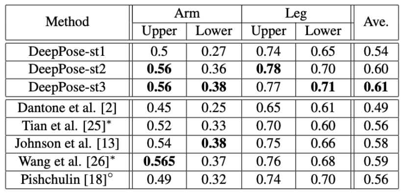
Fig 1. DeepPose: Results of DeepPose Cascading Stage Model vs Contemporaries [1].
At the time, DeepPose was a strong achievement, however, it still had its challenges. The model is small by today’s standards, and had some common failure cases, such as flipping the left and right side of predictions when the image subject was photographed from behind. DeepPose clearly did not “solve” pose estimation, and evolution was still very necessary.
MultiPose
Although DeepPose was remarkable for its significant improvement to pose estimation, it was designed to estimate the pose of a single person per-image. The next logical step was to devise an algorithm to estimate the poses of multiple individuals in a single image. One such model was developed by G Papandreou et al [2]; since the model lacks a name, it will simply be referred to as MultiPose. MultiPose was developed in response to a number of factors, including the success of deep neural networks in pose estimation, the release of the COCO person keypoints dataset, which, as previously mentioned, included a large number of multi-person scenes, and the developments in fast object detection, specifically Faster RCNN.
MultiPose was developed as a two-stage algorithm: first, Faster RCNN would be used to form bounding boxes around people in the image. This effectively was a direct reuse of Faster RCNN for object detection, with only one object class (people) being detected. The second stage was where the primary advancements were made. Given each person bounding box from the first stage, key points were estimated by a joint classification and regression algorithm. The classification aspect classified each point in the cropped region as being within some radius \(R\) of one of the 17 keypoints, and this association was called a heatmap in the paper. The regression was not, in fact, a direct regression to the keypoint locations. Rather, each pixel, in addition to receiving a classification, estimated the vector from its location to the keypoint it was associated with. This sort of pose estimation was known as a top-down approach, where a person was detected before pose was estimated. At the time, this was notably less common than its alternative: the bottom-up approach. This method estimated pose via part detectors, then used inference to group the keypoints into people.
The details of the classification side are as follows. After receiving the bounding box from the person detector, the box was expanded to have a fixed aspect ratio. Notably, this operation performed no distortions to the image aspect ratio, since the height or width of the bounding box was directly enlarged, rather than scaled. This transformed box was then scaled by 1.25 times (as well as a random factor from 1 to 1.5 for data augmentation). The crop for pose estimation was made from this expanded box, then the height was fixed to 353 pixels, and width to 257 pixels.
This new crop is fed into a CNN using ResNet-101 as its backbone. The CNN is fully convolutional. At the output layer, instead of using the fully connected layers of the base ResNet, a 1x1 convolutional layer with 3 output channels per keypoint (for a total of 17 * 3 = 51 channels) is used. The first 17 channels—referred to as the heatmaps—represent the a binary classification for whether a pixel is within radius \(R\) of a keypoint \(k\), ie \(h_k(x_i)=1\) if \(\|x_i-l_k\|\leq R\), where \(l_k\) is the estimated keypoint location. The remaining 34 channels—referred to as the offsets—represent the estimated vector from the pixel to the associated keypoint, forming a vector field.
Following this 1x1 convolution, atrous convolution was used with 3 output channels per keypoint and an output stride of 8 pixels, followed by bilinear interpolation, scaling the output back to the 353x257 crop. The upsampled output then fuses the heatmaps and offsets as follows:
\[f_k(x_i) = \sum_j \frac{1}{\pi R^2} G(x_j + F_k(x_j) - x_i) h_k(x_j) \tag{4}\]where \(G\) is the bilinear interpolation kernel. This function effectively sums the expected keypoint locations from each pixel associated with that keypoint, forming a highly precise activation map.
This model was trained using two output heads, corresponding to the heatmaps and offsets. The heatmap loss \(L_h\) was calculated as the log loss for each position and keypoint combination, while the offset loss was calculated as:
\[L_o(\theta) = \sum \limits_{k=1:K} \sum \limits_{i:\|l_k-x_i\|\leq R} H(\| F_k(x_i) - (l_k - x_i) \|) \tag{5}\]where H(u) is the Huber robust loss: (\(u^2\)/2 for \(abs(u)\) ≤ δ and δ(\(abs(u)\) - δ / 2) otherwise, for some δ)
\(l_k\) is the k-th keypoint location. Loss for offsets is only calculated for positions actually within the radius \(R\) of the keypoint. The final loss, then was
\[L(\theta) = \lambda_h L_h(\theta) \lambda_o L_o(\theta) \tag{6}\]where \(\lambda_h\) and \(\lambda_o\) were scaling factors for balance—the values used in MultiPose were \(\lambda_h = 4\) and \(\lambda_o = 1\). This loss was complicated when considering other people’s keypoints may appear in the background of a bounding box in crowded circumstances. For this circumstance, the heatmap loss only considered the keypoints associated with the person in the foreground.
Two final features of MultiPose relate back to the use of the person detector, with the fist being an alternative method of pose scoring. Instead of relying on the base model of Faster RCNN for drawing bounding boxes, a new score was developed. This score was calculated as the average maximal activation for each keypoint:
\[\text{score}(\mathcal{I}) = \frac{1}{K} \sum\limits^K_{k=1} \max\limits_{x_i} f_k(x_i) \tag{7}\]This modification helped guide the bounding boxes to provide more valuable context clues, and generally focus the objective on maximizing joint location confidence. The final feature was the use of a variant of non-max-suppression. Instead of using IOU to eliminate overlapping bounding boxes, the similarity score was calculated using OKS—the same evaluation metric mentioned earlier. This change was primarily useful in differentiating between two people in close proximity, or two poses for the same person—both might have a high IOU, but two poses for the same person are more likely to have a higher OKS, than two poses for separate, but close, people.
MultiPose took full advantage of the recent release of COCO, training the model both on the base COCO dataset, as well as a dataset supplemented by in-house data. The results were competitive with prior state-of-the-art results for COCO, such as CMU-Pose and Mask-RCNN, for both the supplemented dataset and the original COCO dataset.
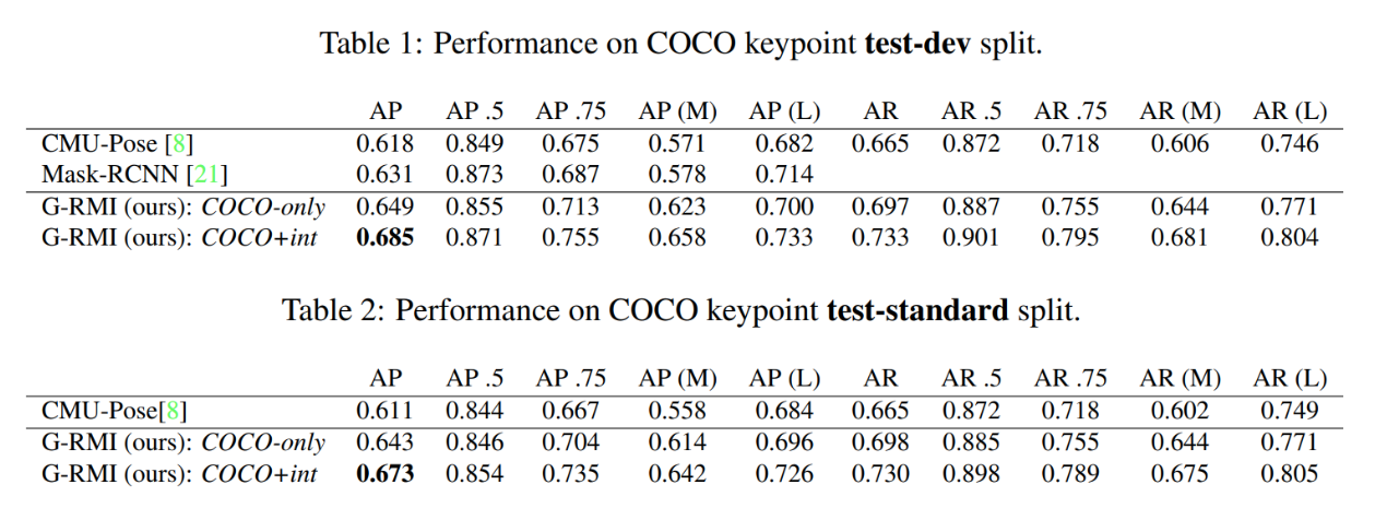
Fig 2. MultiPose: Results of MultiPose vs Contemporary State-of-the-Art Multi-person Pose Estimators [2].
Not only was MultiPose competitive, it outperformed the prior models in nearly all categories, with the one exception being AP .5. While there were still more advancements to come, MultiPose demonstrated several important techniques and methods in pose estimation—particularly the heatmap estimation—which would be refined by future work.
DARK
Distribution-Aware Coordinate Representation for Human Pose Estimation (DARK) proposes a new method for key point prediction that increases validation on existing heatmap based pose models as DARK is model-agnostic and can be easily integrated with such architectures [3]. DARK utilizes heatmaps for key point prediction by predicting heatmaps around the predicted key points and using the heatmaps to find the best pixel for the key point. The proposed heat map based models follows a simple architecture:
- crop and resize the input image around the detected human
- significantly reduce the resolution of the image (to improve computational efficiency)
- pass the reduced image into a CNN to predict heatmaps around each key point
If training:
- compute the loss with the ground truth heatmaps during training
If testing:
- resolution recovery and reshape to original image size
- calculate the key points from the predicted heatmaps To train the model by calculating the loss between ground truth heatmaps, the model requires that all ground truth images are converted from key point predicted images to heatmaps around the key point positions.
Dark addresses the standard coordinate decoding method (i.e. deriving the key point position from a heat map) which takes a heat map and identifies the coordinates of the maximal (\(m\)) and second maximal (\(s\)) activation. It then uses the following formula to produce the coordinate of the point:
\[\mathbf{p} = \mathbf{m} + 0.25\frac{\mathbf{s}-\mathbf{m}}{\|\mathbf{s}-\mathbf{m}\|_2} \tag{8}\]This equation produces a key point at the maximal heat map pixel location shifted by ¼ toward the second maximal position. The final position in the original image is produced by the following equation where \(\lambda\) is the resolution reduction ratio.
\[\mathbf{\hat{p}} = \lambda \mathbf{p} \tag{9}\]DARK claims that this standard coordinate prediction system is flawed because the maximum activation in the predicted heatmap is not the actual position of the key point but rather merely a coarse location of it.
To overcome this, DARK’s coordinate decoding method utilizes the predicted heat map’s distribution structure to discover the maximum activation position. DARK assumes that both the predicted and ground truth heat map follow a 2D gaussian distribution. Using this assumption, they model the heat map with the following two equations (10 being the generic equation and 11 being an equivalent yet simplified version) and use the second one (11) to predict \(\mu\), the corresponding key point position:
\[\mathcal{G}(\mathbf{x};\mathbf{\mu},\Sigma) = \dfrac{1}{(2\pi)|\Sigma|^{\frac{1}{2}}}\exp(-\frac{1}{2} (\mathbf{x}-\mathbf{\mu})^T \Sigma^{-1} (\mathbf{x}-\mathbf{\mu})) \tag{10}\] \[\mathcal{P}(\mathbf{x};\mathbf{\mu},\Sigma) = \ln(\mathcal{G}) = -\ln(2\pi) - \frac{1}{2}\ln(|\Sigma|) - \frac{1}{2}(\mathbf{x}-\mathbf{\mu})^T \Sigma^{-1} (\mathbf{x}-\mathbf{\mu}) \tag{11}\]To solve for \(\mu\) they utilize the underlying distribution’s structure as \(\mu\) is an extreme point in the distribution, thus the first derivative at \(\mu\) is trivially:
\[\left. \mathcal{D}'(\mathbf{x}) \right|_{\mathbf{x}=\mathbf{\mu}} = \left. \frac{\partial\mathcal{P}^T}{\partial \mathbf{x}} \right|_{\mathbf{x}=\mathbf{\mu}} = \left. -\Sigma^{-1}(\mathbf{x}-\mathbf{\mu}) \right|_{\mathbf{x}=\mathbf{\mu}} = 0 \tag{12}\]Using the first derivative as well as the second derivative defined below (13) they compute \(\mu\) using the following equation (14):
\[\mathcal{D}''(\mathbf{m}) = \left. \mathcal{D}''(\mathbf{x}) \right|_{\mathbf{x}=\mathbf{\mu}} = -\Sigma^{-1} \tag{13}\] \[\mathbf{\mu} = \mathbf{m} - (\mathcal{D}''(\mathbf{m}))^{-1}\mathcal{D}'(\mathbf{m}) \tag{14}\]Once obtaining \(\mu\) they also apply equation (9) from above to predict the coordinate in the original image space. DARK’s method determines the underlying maximum more accurately by exploring the heat map’s statistics in its entirety. Furthermore, it is computationally efficient as it only computes the first and second derivative with respect to one pixel per heat map.
DARK’s proposed algorithm relies on a crucial assumption: the predicted heatmaps follow a gaussian distribution. However, most of the time heatmaps predicted by models do not possess a well distributed gaussian structure compared to the training heatmap data. To overcome this, DARK suggests modulating the heatmap distribution by using a gaussian kernel K with the same variation as the training data to smooth out multiple peaks in the heatmap \(h\) by using the following equation where ⊛ denotes the convolution operation.
\[\mathbf{h}' = K ⊛ h \tag{15}\]To preserve the magnitude of the original heatmap \(h\), simply scale \(h'\) so that its maximal activation is the same as \(h\)’s using:
\[\mathbf{h}' = \dfrac{\mathbf{h}' - \min(\mathbf{h}')}{\max(\mathbf{h}') - \min(\mathbf{h}')} * \max(\mathbf{h}) \tag{16}\]By using this distribution modulation, DARK’s experiments validated further performance improvements of their coordinate decoding method.
One final change DARK makes to the traditional heatmap based models is a change in the coordinate encoding process. The standard method leads to inaccurate and biased heatmap generation which they overcome by placing their heatmaps’ center at a non-quantised location which represents the accurate ground-truth coordinate.
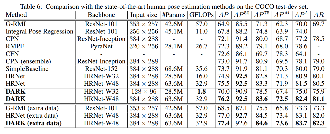
Fig 3. DARK: Results of DARK vs Contemporary Pose Estimators [3].
DARK was tested on two popular datasets, COCO and MPII, where they saw significant improvements in performance relative to other state-of-the-art models. Thus, DARK is an innovative method for improving accuracy within heatmap based human pose prediction models and can easily be applied to existing models without making changes to the model’s structure or computational efficiency.
References
[1] A. Toshev and C. Szegedy, “DeepPose: Human Pose Estimation via Deep Neural Networks.” in 2014 IEEE Conference on Computer Vision and Pattern Recognition, 2014.
[2] Papandreou et al. “Toward Accurate Multi-person Pose Estimation in the Wild.” (2017).
[3] Zhang et al. “Distribution-Aware Coordinate Representation for Human Pose Estimation.” (2019).